2.0 Greenhouse Gas Basics

• 2.1 What Are GHGs?
• 2.2 GHGs versus Criteria Pollutants
• 2.3 Mitigation versus Adaptation
• 2.4 Why Is Reducing GHGs Important?
• 2.5 Impacts on Transportation
• 2.6 Contribution of U.S. Transportation Sector to GHGs
• 2.7 Scope of Emissions Included in a Transportation Inventory
• 2.8 Establishing a Baseline of Emissions
• 2.9 Transportation GHG Reduction Strategies
• 2.10 Case Study: Relative Magnitude of Emissions from State Transportation Sources
• 2.11 Relationship Between GHGs and Other Environment and Sustainability Issues

2.1 What Are GHGs?

Greenhouse gases (GHGs) are those that absorb and emit infrared radiation in the wavelength range emitted by Earth. GHGs emitted by human activity include carbon dioxide (CO₂), methane (CH₄), nitrous oxide (N₂O), chlorofluorocarbons (banned in 1996 by the Montreal Protocol), and hydrofluorocarbons (HFCs).

GHGs contribute to warming through the greenhouse effect, a process wherein atmospheric gases trap reflected sunlight, keeping the earth warm. The chemical composition of the atmosphere determines the wavelengths of light that can pass through the atmosphere and thus the degree of warming. CO₂ and CH₄, for example, absorb and retain certain wavelengths of energy. The more heat-retaining molecules present in the atmosphere, the warmer the planet becomes.

The resulting impact on warming (per unit mass) associated with each pollutant type can be expressed in terms of global warming potential (GWP). GWP factors are used to convert other emissions to CO₂ equivalents (CO₂e). Emissions of CO₂e are usually expressed in metric tons (mt) or million metric tons (mmt), where a metric ton [1,000 kilograms (kg)] is equivalent to 2,205 pounds. GWP considers a pollutant’s effects over a particular timeframe, typically 100 years, to account for the residency time of the gas or particle in the atmosphere as well as its heat-trapping potency.

Table 2.1 shows the latest available estimates for the GWP of greenhouse gases and their approximate contribution to the U.S. transportation inventory, expressed as a percent of total CO₂e. N₂O levels have dropped substantially in recent decades due to exhaust emissions controls, and CO₂ now represents 96 percent of direct emissions.

Table 2.1 Estimated GWP of GHGs and Contribution to U.S. Transportation Inventory

Chemical Compound	Lifetime (years)	100-Year Global Warming Potential	20-Year Global Warming Potential	% Increase in Atmosphere, 1750—2011/2013	Approximate Contribution to U.S. 2016 Transportation Inventory (%)
Carbon Dioxide (CO2)	n/a	1	1	41%	96.1%
Methane (CH4)	12	28	84	152–170%	0.9%
N2O	121	265	264	20%
Fluorinated gases	n/a	n/a	n/a	n/a	2.4%
HFC-134a	13	1,430	3,710	n/a	n/a
HFC-152a	n/a	124	n/a	n/a	n/a
HFO-1234yf	n/a	4	n/a	n/a	n/a

HFC = hydrofluorocarbon; HFO = hydrofluoroolefin

Sources:
Lifetime and GWP: Working Group I Report, Chapter 8, Appendix 8.A (note: protocols may differ from latest science) [Intergovernmental Panel on Climate Change (IPCC), 2014]. HFC-152a and HFO-1234yf from U.S. Environmental Protection Agency (EPA) (https://www.epa.gov/mvac/refrigerant-transition-environmental-impacts).
Percent increase: Various sources as referenced on Wikipedia, accessed February 2019.
Contribution to transportation inventory: Inventory of U.S. Greenhouse Gas Emissions and Sinks (U.S. EPA, 2018). HFC-134a is a common automotive refrigerant [first introduced to replace ozone-depleting chlorofluorocarbon (CFC-12), which cannot be used in new light-duty vehicles manufactured in model years 2021 and beyond due to its climate forcing impacts]. HFC-152a and HFO-1234yf are acceptable substitutes for new or retrofitted vehicles as determined by the U.S. EPA.

2.2 GHGs versus Criteria Pollutants

Although GHGs have different effects and are regulated through different mechanisms than other pollutants, they are often considered in conjunction with a State department of transportation’s (DOT’s) air quality activities, which target criteria pollutants and precursors. Criteria pollutants include ozone, sulfur dioxide, carbon monoxide (CO), particulate matter, lead, and nitrogen dioxide (NO₂). Some of these are emitted directly from vehicle exhaust, and some are formed by chemical reactions of exhaust components.

Criteria pollutants affect local and regional air quality and are regulated at the Federal level mainly on the basis of human health impacts from direct exposure. The Clean Air Act sets national ambient air quality standards for criteria pollutants. In contrast, GHGs have global effects; where they are emitted does not matter. There currently are Federal regulations for emission rates per vehicle, in the form of GHG tailpipe standards harmonized with fuel economy standards, but not for total emissions or ambient concentrations. The U.S. EPA provides information on criteria air pollutants.

2.3 Mitigation versus Adaptation

Although climate change is often addressed under one umbrella, planning for climate change encompasses two distinct activities:

• Mitigation efforts to reduce emissions, actively remove GHGs from the atmosphere through sequestration, or manage the effects of GHGs through geoengineering.
• Adaptation efforts to respond to the changing environment so as to lessen impacts on infrastructure and travel. For transportation, this typically means considering how infrastructure can be made more resilient to the effects of today’s extreme weather as well as to future weather patterns associated with a changing climate.

The focus of this guide is mitigation; other resources have been developed to help State DOTs adapt to climate impacts and improve the resilience of the transportation system.

2.4 Why Is Reducing GHGs Important?

Although CO₂ levels fluctuate over tens of thousands of years, the current level of CO₂ is much higher—and has increased much more rapidly—than ever previously observed (Figure 2.1). Current CO₂ emissions are expected to remain in the atmosphere for decades, if not centuries.

Figure 2.1 Atmospheric CO₂ Concentrations over the Past 800,000 Years

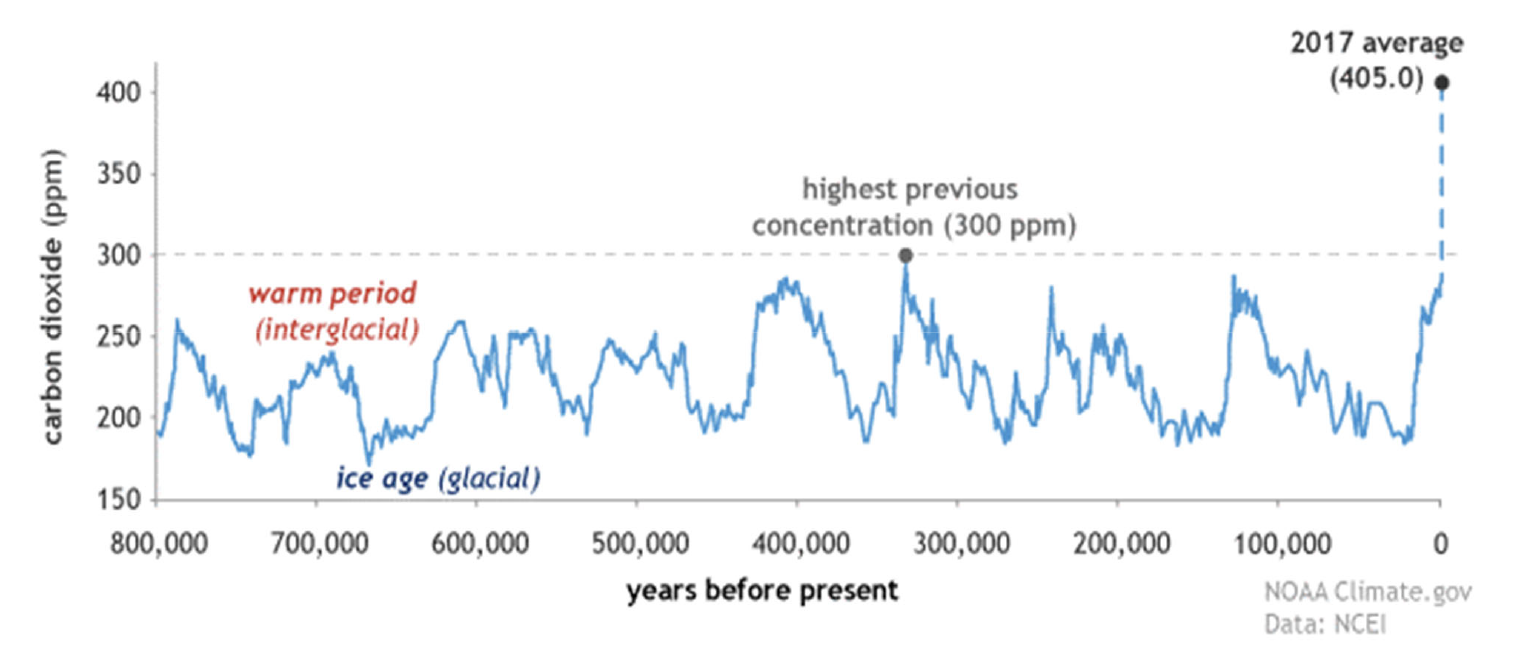
Source: National Centers for Environmental Information (NCEI) and National Oceanic and Atmospheric Administration Climate.gov.

One result of increased CO₂ levels is extreme weather. The occurrence of extreme weather events has increased markedly since the mid-1990s. Research points to continued change in temperature and precipitation across the U.S., with impacts unevenly distributed spatially. Extreme precipitation is expected to increase across the U.S., while temperatures will rise most at high latitudes (Figure 2.2, Figure 2.3). Agricultural yields are projected to drop markedly in much of the Midwest but increase in the Pacific Northwest. According to the U.S. Global Change Research Program (U.S. GCRP), energy expenditures will likely increase across the South (U.S. GCRP, 2018).

Figure 2.2 Projected Change in Coldest/Warmest Temperatures

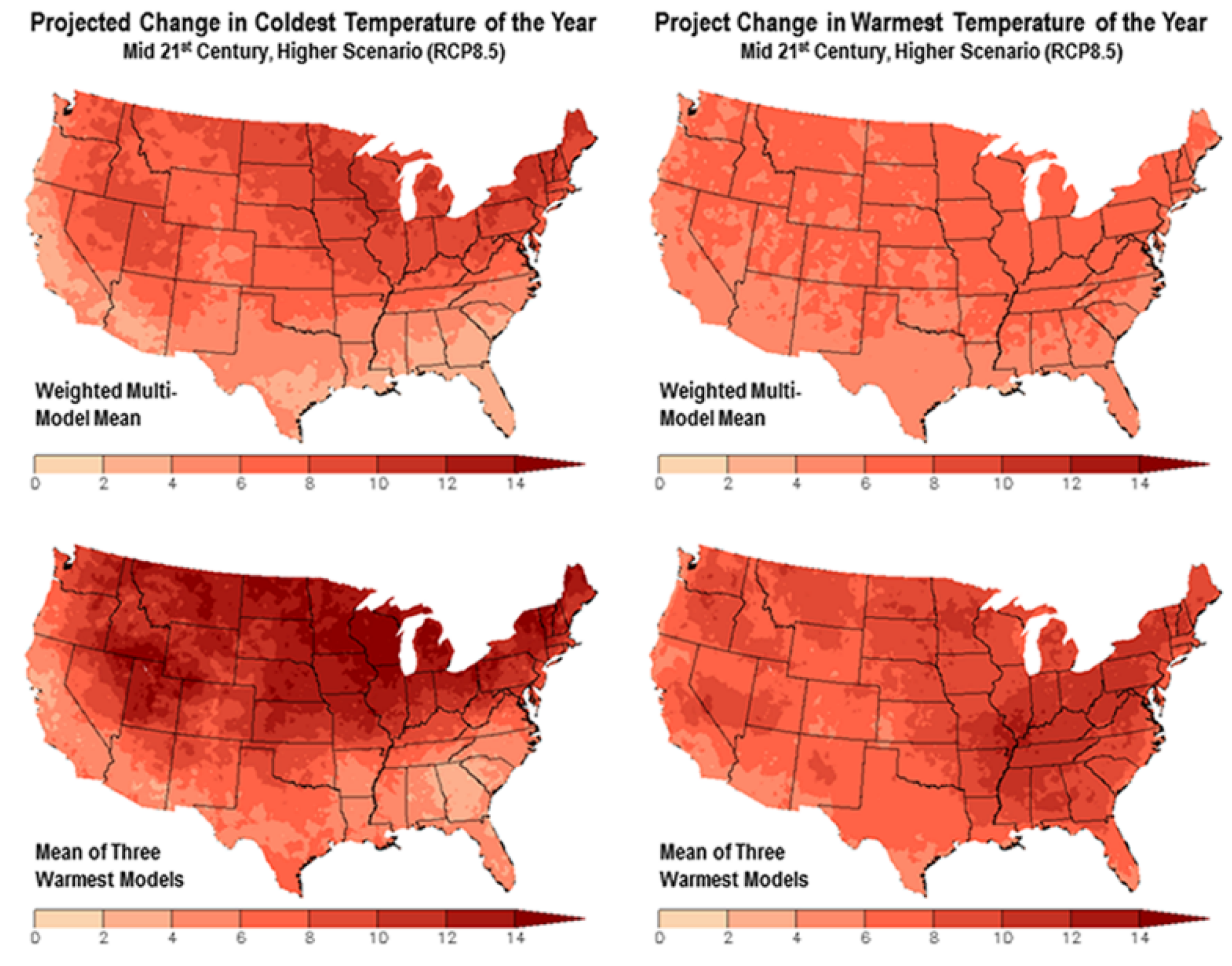
Source: U.S. GCRP, 2018.

Figure 2.3 Projected Change in Daily, 20-Year Extreme Precipitation Under Lower and Higher GHG Emissions Scenarios

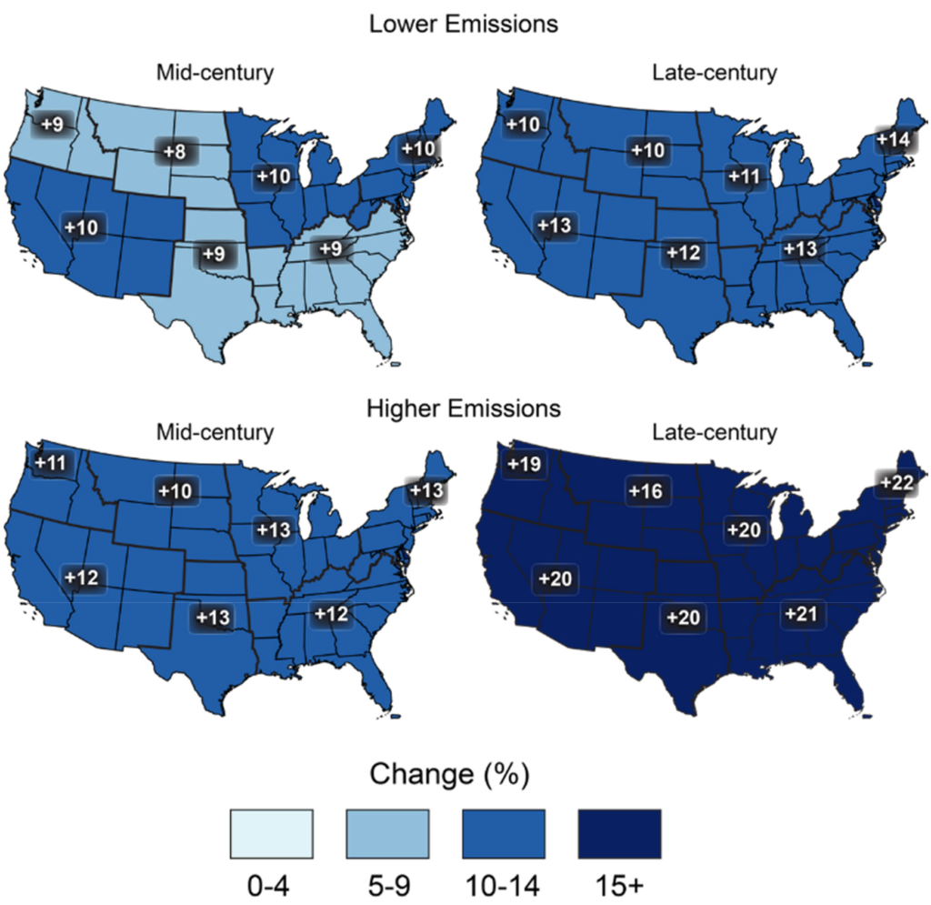
Source: U.S. GCRP, 2018.

Given current emissions and warming trends, the average temperature of the planet may increase by 1.5°C by 2040 and close to 2.0°C by 2060. As shown in Figure 2.4, holding temperature increases to below 2.0°C—a threshold limit for some of the most disruptive environmental effects—will require net zero CO₂ emissions by at least 2055 and significant reduction of non-CO₂ by at least 2030 (IPCC, 2014).

Figure 2.4 CO₂ Scenarios to Limit Warming

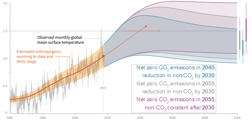
Source: IPCC, 2014.

As such, international accords and local policies have aimed for aggressive GHG reduction targets of at least 80 percent by 2050. In a recent international agreement, the Paris Accord, 184 nations were party to a set of agreements aiming to keep the increase in global average temperature below 1.5°C. In the U.S., at least 22 States and the District of Columbia have set statewide emissions targets. Many cities in the U.S. have also set goals and joined alliances to meet aggressive GHG reduction targets.

2.5 Impacts on Transportation

Table 2.2 illustrates the potential impact of extreme weather due to climate change on transportation infrastructure. Although there is substantial variation in potential magnitude, depending on the emissions scenario and the model used, disruptive impacts may be significant (U.S. GCRP, 2018). There also are several potential positive impacts for infrastructure, including reduced snow and ice removal costs, reduced winter hazards, and longer periods of ice-free port and marine shipping operations [National Academy of Sciences (NAS), 2008].

Table 2.2 Transportation Infrastructure Impacts of Climate Change

Impact Type	Potential Magnitude	Transportation Infrastructure Impacts
Sea level rise	1’–8.2’ by 2100	Flooding and storm surge— coastal transportation facilities
More intense storms	50–300% increase in extreme precipitation events by 2100	Overtopping and erosion of roads, bridges, rail lines in river valleys Need for evacuation routes
Excessive summer heat	+2.5–2.9 °F by mid-century +5.0–8.7 °F by late-century	Pavement and rail integrity
Prolonged droughts		Lower water levels in rivers/shipping channels Wildfires—road closures

Source: U.S. GCRP, 2018.

There may also be non-infrastructure impacts to the transportation network. Air pollution, exposure to disease vectors, reduction in animal habitats and biodiversity, ocean acidification, destruction of crops and fisheries, and changes in the location of population and economic activities all may generate spatial and temporal shifts in travel demands.

Inherent in these shifts are several key threats relevant to the work and mission of State DOTs (U.S. GCRP, 2018):

• Facilities at risk of permanent closure: Many transportation facilities are at risk of permanent closure due to rising sea levels; already, 13 of the nation’s largest airports have runways within the reach of moderate to high storm surge.
• Interruption of freight and passenger travel: Even if facilities are not forced to close, they can be disrupted by increasing rates of wildfire, flooding, and severe weather. These events increase the costs of maintenance and interfere with planning and logistics. High temperatures and increased thermal cycles can cause expansion joints on freeways and bridges to deteriorate more rapidly (Meyer, Amekudzi, and O’Har; 2010).
• Safety and health risks: There are real costs in human lives associated with extreme events, including flooding, landslides, high winds, ice storms, dust storms, and wildfires.
• Increasing public demand for action: As public support for action on climate change increases, State DOTs will be expected to provide leadership on statewide policy initiatives.^[1]

2.6 Contribution of U.S. Transportation Sector to GHGs

Direct emissions from transportation sources represent just under 30 percent of U.S. GHG emissions (Figure 2.5). Light-duty vehicles account for almost 60 percent of these emissions, with approximately 20 percent from freight trucks, 9 percent from aircraft, and the remainder from other modes. Overall, on-road travel makes up over three-quarters of transportation emissions.^[2]

Figure 2.5 U.S. Transportation GHG Emissions and Type

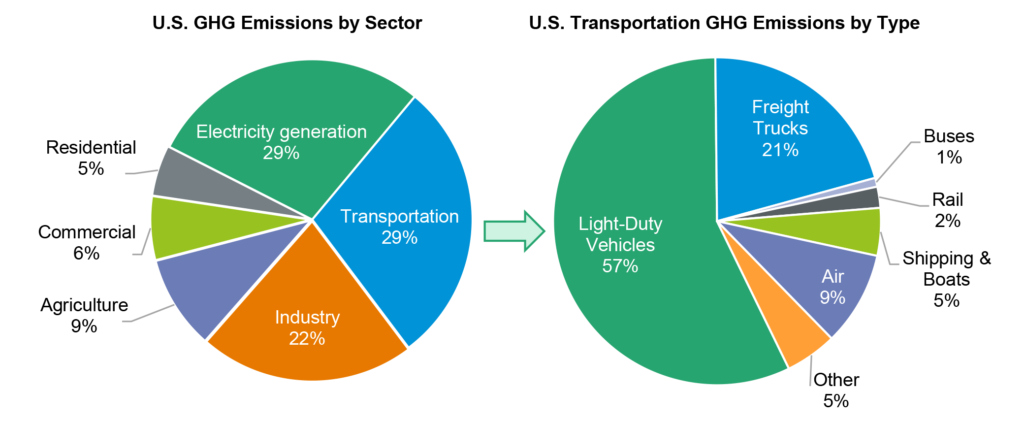
Source: U.S. EPA, 2018; calculations based on U.S. Department of Energy (DOE), 2019.

Shifts in the fuels used for electricity generation have led U.S. GHG emissions to decline overall since 2007. In contrast, direct transportation GHGs in the U.S. have been roughly flat since the late 1990s at around 2,000 million metric tons (Figure 2.6). CO₂ represents the vast majority of direct transportation emissions; fluorinated gases used as refrigerants make up about 2.4 percent, while N₂O and CH₄ together are less than 1 percent.

Figure 2.6 GHG Emissions 1990–2017 by Type

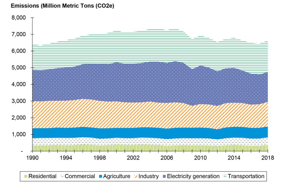
Source: U.S. EPA, 2018.

There are several types of emissions in the transportation sector. “Operating,” or “direct,” emissions include emissions from fuel combustion to move the vehicle. “Nonoperating” emissions include upstream emissions associated with fuel production; embodied emissions associated with construction and disposal of the vehicles; and embodied emissions associated with infrastructure construction and maintenance. Considering both operating and nonoperating emissions together results in a “life-cycle emissions” value. For transportation, the life-cycle emissions values are significantly higher than simple operating emissions—adding 63 percent to emissions from on-road sources (Figure 2.7).

Figure 2.7 Operating and Nonoperating Emissions from Transportation

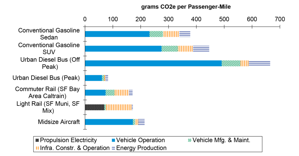
Source: Chester and Horvath, 2009. “Conventional gasoline sedan” is a 2005 Toyota Camry and “conventional gasoline sport utility vehicle” is a 2005 Chevrolet Trailblazer. “Midsize aircraft” is a Boeing 737. All vehicles are at average occupancy levels.

2.7 Scope of Emissions Included in a Transportation Inventory

2.7.1 Scope 1, Scope 2, and Scope 3 Emissions

Anyone following GHG inventory protocols, such as the Global Protocol for Community-Scale Greenhouse Gas Emission Inventories (GPC) (World Resources Institute, ICLEI, and C40 Cities) will soon encounter the terms “Scope 1,” “Scope 2,” and “Scope 3” emissions:

• Scope 1 emissions are generated by sources within the organization or jurisdiction (State or municipality) boundary.
• Scope 2 emissions occur as a consequence of the use of grid-supplied electricity, heat, steam and/or cooling within the organization or jurisdiction boundary.
• Scope 3 emissions include all other GHG emissions that occur outside the boundary as a result of activities taking place within the boundary. Examples include employee commuting (for a DOT agency inventory); emissions associated with extraction, production, and transport of fuels; or emissions released in the manufacturing of construction materials that are used within the State but manufactured outside the State (for a statewide inventory).

Carbon footprinting for a DOT’s operations will typically include Scope 1 and Scope 2 emissions and may include Scope 3 emissions. For a statewide inventory, typically only Scope 1 and Scope 2 emissions would be included. However, States may choose to report Scope 3 emissions to provide additional information (see below for discussion of “direct versus life-cycle” emissions).

2.7.2 Transportation versus Other Sector Emissions

A minor issue for base-year inventories, but one that will increase in importance in the future, is the common approach to reporting emissions by economic sector. This approach is straightforward when considering petroleum fuels used for the vast majority of current transportation sector energy. However, the introduction of electric vehicles (EVs) creates complications, since electricity emissions (including those generated by EVs) are typically reflected in nontransportation sectors. This can lead to a situation where the transportation portion of the GHG inventory does not reflect emissions from EVs, giving a false picture that EVs will produce zero transportation emissions in the future, when these emissions should be reflected in increased emissions from the electricity sector. Many of the upstream emissions associated with petroleum and biofuels also are reflected in other sectors’ emissions data.

Agencies should be aware of the protocols used for reporting of emissions within their State. It may be necessary to define multiple levels of reporting so that emissions from electrification can be accurately reflected in an evaluation of transportation-specific strategies.

2.7.3 Direct versus Life-Cycle Emissions

A narrow focus on Scope 1 and Scope 2 emissions will also exclude “upstream” emissions generated with fuel production and distribution. Again, this is not a major problem when looking just at today’s petroleum-based fuels. However, it does create a problem when evaluating alternative fuels, such as ethanol and biodiesel, that generate similar direct emissions to petroleum but have very different life-cycle effects. Simply comparing tailpipe emissions will not accurately reflect these effects. At the other end of the spectrum, excluding biofuels from an inventory or assessment (as has been done in some studies) can paint an unfairly optimistic view of strategies to shift to these fuels. Also, reporting of electricity emissions is inherently done on a life-cycle basis (or at least most of the life-cycle—fuel production and transport to the generating station may be excluded) since there are no “direct” emissions from the vehicle. A focus only on operating emissions also does not consider emissions embodied in materials used in transportation infrastructure and vehicles. Again, multiple levels of reporting may be required to be consistent with State protocols while also providing a balanced assessment of alternative fuels.

Emission factor models, including the Motor Vehicle Emission Simulator (MOVES) and Emission Factor (EMFAC), only report direct or “tailpipe” emissions. Other data and tools, such as the Greenhouse Gases, Regulated Emissions, and Energy Use in Transportation (GREET) model, are needed to estimate life-cycle emissions. More information on emission factor models and their capabilities is provided in Appendix B.

2.8 Establishing a Baseline of Emissions

Future changes in emissions are typically measured with respect to a historical reference point. As such, measuring forecasted impacts of GHG mitigation strategies requires setting a baseline that represents expected outcomes if no further actions are taken beyond today’s policies. Baselines can be extrapolated from historical trends or developed using models (e.g., travel demand forecasting). It is important to recognize the uncertainty inherent in baselines due to the presence of external unknowns such as oil prices or consumer preferences. Policies driving vehicle fuel efficiency and technology, including Federal Corporate Average Fuel Economy (CAFE) and California Zero-Emission Vehicle (ZEV) standards, can also evolve and affect future baseline projections. Methods for projecting baseline transportation sector emissions are discussed in Section 10.0 with some examples shown in Section 3.0.

The U.S. DOE provides estimates of emissions by State for the most recent reporting year. The U.S. DOE Annual Energy Outlook (AEO) provides projections of national emissions. The AEO 2019 Reference Case projects transportation emissions from 2018 to 2050 and anticipates that light-duty vehicle emissions will decline by about 25 percent (Figure 2.8). The projection also indicates a slight growth in freight truck emissions, a slight decline in both domestic and international freight rail/shipping, and significant growth in aircraft emissions due to increasing air travel.

Figure 2.8 Projected U.S. Transportation Emissions, 2018 to 2050

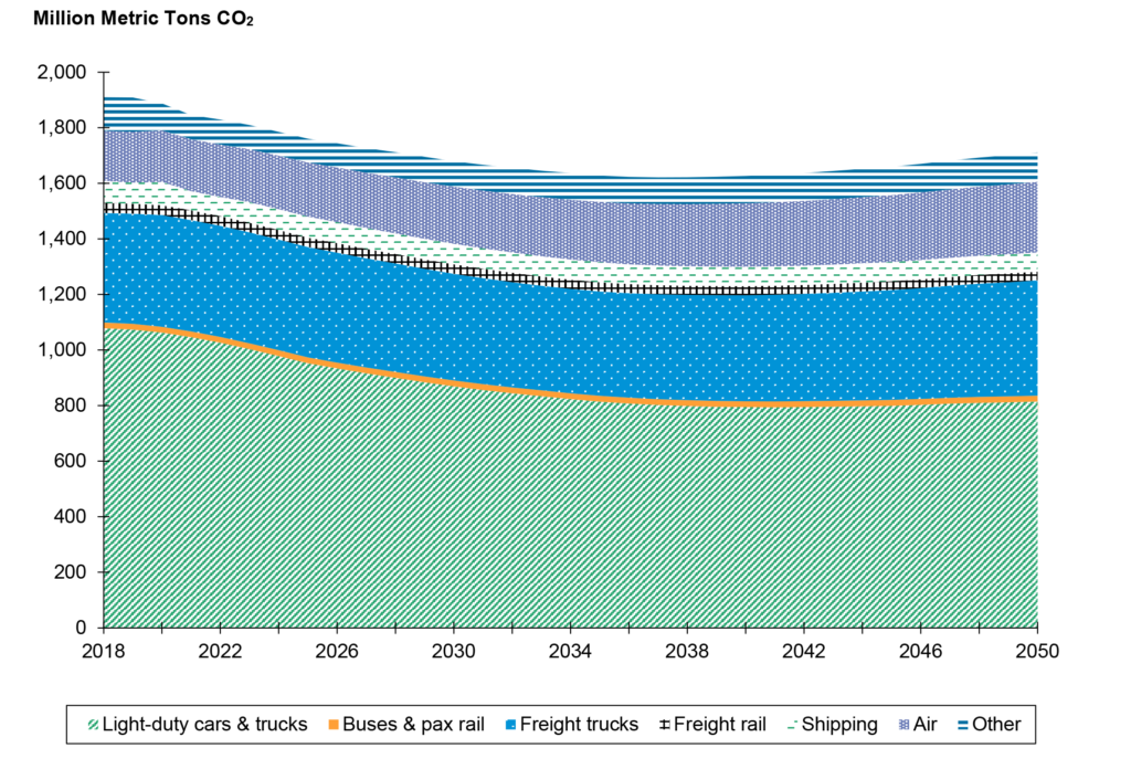
Source: U.S. DOE, 2019; Reference Case.

2.9 Transportation GHG Reduction Strategies

There are several primary strategies for GHG reduction in transportation:

• Reducing the carbon intensity of fuels.
• Making vehicles more fuel efficient.
• Improving the efficiency of transportation system operations.
• Reducing the amount of travel or shifting it to less carbon-intensive modes.
• Reducing emissions from material production, construction, and maintenance of the transportation system through lower-carbon materials and processes or more durable applications.
• Offsetting carbon emissions (see “What Are Carbon Offsets?”).

The areas in which a State DOT has the most influence are in system efficiency; reduction of travel using carbon-intensive modes; and reduction in emissions associated with construction, maintenance, and operations, including the emissions footprint of materials as well as equipment and operations. However, the DOT may also be a partner in other strategies, such as deploying infrastructure to support EVs or low-carbon fuels.

2.10 Case Study: Relative Magnitude of Emissions from State Transportation Sources

This case study illustrates the relative magnitude of GHG emissions from users of the transportation system (passenger and freight vehicles) compared to a typical DOT’s current activities to construct and maintain the system as well as the DOT’s administrative operations (buildings and fleets). Data from Florida, Maine, Massachusetts, Minnesota, Maryland, Oregon, Texas, Vermont, and Washington State are used to provide a picture of a hypothetical “composite” State. The specifics may vary by State, but the general scale of emissions should be similar.

In this example hypothetical State, the vast majority of emissions—about 50 million metric tons CO₂e annually—are generated by system users (Figure 2.9). This is a life-cycle estimate that includes direct vehicle emissions from the combustion of gasoline and diesel fuels for passenger and freight transport on the entire State transportation network, as well as upstream emissions associated with fuel production and distribution. Approximately 6 percent of emissions—about 3 million metric tons—is generated from materials and fuels used in the construction, maintenance, and operation of the State’s highway infrastructure. About two-tenths of a percent of emissions, or 100,000 metric tons, are generated through State DOT administrative operations, including office buildings and passenger vehicles. While infrastructure and administration emissions are relatively small compared to total transportation system user emissions, they are also the sources over which the DOT has the most direct control.

Figure 2.9 Example State: Scale of GHG Emissions by Type

Source: Calculations by Good Company. Users of the system figure based on data from Florida, Maine, Massachusetts, Minnesota, Maryland, Oregon, Vermont, Washington, and Texas DOT sustainability/GHG inventory reports and system characteristics, including vehicle miles traveled (VMT), population, lane miles, and fuel mix. State highway system figure based on data from these States’ budget documents and U.S. Environmentally-Extended Input-Output (USEEIO) Model factors. Administration figure based on data from Florida, Minnesota, Oregon, Washington, and Texas DOT sustainability/GHG inventory reports. All estimates are life-cycle emissions.

This example considers a typical State’s activities at the current time, when the transportation system is largely built out and the “state highway system” activities are largely maintenance related. Considering the life-cycle contribution of all roadways, including new construction, could result in much greater emissions. For example, data from Chester and Horvath (2009), as presented in Figure 2.7 of this guide, suggest that emissions from construction and maintenance activities add about 20 to 25 percent of the emissions from light-duty cars and trucks traveling on the roadways when prorated on a per vehicle lifetime basis.

2.11 Relationship Between GHGs and Other Environment and Sustainability Issues

GHG reduction strategies often, although not always, overlap and align with strategies directed at other sustainability-related objectives. For example:

• GHG reduction can be achieved by reducing energy use, supporting energy independence goals.
• GHG reduction measures often coincide with measures to reduce emissions of criteria air pollutants and precursors.
• GHG reduction and climate mitigation is widely considered a critical component of sustainability initiatives.

Many GHG reduction strategies provide substantial “co-benefits,” such as mobility, safety, land preservation, equity, and public health. For example, strategies to improve walking, bicycling, and public transportation and shift trips out of personal vehicles can improve mobility for transit-dependent populations, improve the safety of these modes, and encourage physical activity.

---

[1]     https://news.gallup.com/poll/231530/global-warming-concern-steady-despite-partisan-shifts.aspx. In this poll from 2018, 43% of respondents say they worry a great deal about climate change, up from 32% in 2015.

[2]     Calculations based on 2019 Annual Energy Outlook (U.S. DOE, 2019).

Previous | Next