4.0 GHG Emissions Analysis
4.1 Relationship Between Plan-Level/Programmatic GHG Assessment and Project-Level Environmental Documentation
4.2 GHG Emissions Sources to Include
4.3 Tools and Methods for Planning-Level GHG Analysis
4.4 Tools and Methods for Project-Level GHG Analysis
4.5 Equity Considerations
4.6 Communicating Findings and Drawing Conclusions
4.7 Mitigation Measures
4.8 Project- or Program-Level GHG Assessment in Relation to GHG Goals or Targets
4.9 Examples in Practice
This section addresses key issues related to greenhouse gas (GHG) emissions analysis to support environmental review, including:
- How and why might a plan-level or programmatic GHG analysis be used to support project-level evaluation? What options are available for assessment at each level?
- What sources of emissions might be included or excluded, and why?
- What tools and methods are available to support quantitative GHG assessment at the planning or programmatic level?
- What tools and methods are available to support quantitative GHG assessment at the project level?
- What equity considerations exist with respect to GHG emissions?
- What are effective ways of communicating findings and drawing conclusions related to GHG emissions?
- What GHG mitigation measures might be considered?
- How can project or program-level GHG assessment inform and support progress towards meeting GHG reduction goals or targets?
- What are some examples of how agencies have addressed GHG emissions in environmental review practice?
4.1 Relationship Between Plan-Level/Programmatic GHG Assessment and Project-Level Environmental Documentation
4.1.1 Why Do Plan-Level (Programmatic) GHG Analysis?
Environmental review is most frequently performed for major projects as part of the project development process. Waiting until the detailed project development and design stage to consider GHG emissions, however, is likely to miss some of the most important opportunities to mitigate GHG emissions. Our nation’s transportation system is the product of decades of cumulative decisions not only in transportation infrastructure and services but also land use patterns and evolving vehicle technologies. Our system provides a high degree of mobility for those able to use personal vehicles, but this mobility has come at the price of a high degree of energy and carbon intensity.
Because our nation’s transportation system is so highly built out, the incremental impact of any individual project decision, or even a 10- or 20-year investment plan, on GHG emissions is likely to be relatively modest. Nonetheless, the systems planning level of decision-making still provides a greater opportunity to influence future emissions relative to individual project decisions. Depending on the circumstances, a plan-level or programmatic analysis of GHG emissions may be referenced in project-specific environmental documentation in addition, or as an alternative, to conducting project-specific analysis of GHG effects. Key questions that are best addressed at a systems planning or programmatic level include:
- What policies and practices can support the application of more efficient and less carbon-intensive transportation technologies, such as electric vehicles (EVs), micromobility, and shared autonomous mobility, to move people and goods?
- How are we prioritizing our transportation dollars – what modes, what types of projects, and in what locations – within the constraints of existing funding sources? How are these priorities likely to increase or decrease carbon-intensive travel activity?
- How can our transportation investments best support existing and desired future local and regional land use patterns? What is the combined effect of transportation and land use decisions on emissions? How can local, regional, and state decision-making be coordinated to reduce emissions?
- What programmatic decisions can support lower-carbon travel options? For example, are policies and design standards in place to routinely incorporate “complete streets” design elements into roadway reconstruction and rehabilitation?
- What programmatic decisions can support lower-carbon construction, maintenance, and operations activities? For example, specifications for low-carbon materials and procurement of energy-efficient equipment.
In addition to addressing emissions at the most influential decision points, a plan- or program-level GHG evaluation can also support efficiencies in project evaluation and documentation. Transportation systems planning alternatives, considered through the long-range planning process, can be evaluated and compared for GHG emissions effects just like project alternatives. Plan-level evaluations may not capture all the details of GHG effects of specific projects, such as multiple, wide-ranging alternatives, an intersection redesign, or the choice of construction materials, but they do provide a look at the combined impacts of multiple projects. If an individual project is included in the set of projects included in a transportation plan evaluated for GHG effects, or at least similar to these projects, the GHG effects of an individual project might be inferred to be a subset of the overall impacts of the plan or program. The Council on Environmental Quality (CEQ) and Federal Highway Administration (FHWA) both support the use of programmatic information in project-level environmental documentation, and some states have also proposed this as a preferred approach (see Sidebar 4-1).
Sidebar 4-1: Support for Program-level GHG Assessment
A number of federal and state agency documents have expressed support for referencing planning or programmatic-level GHG assessments within project-level environmental documentation. (Unless explicitly stated, this support does not necessarily preclude the conduct of a project-specific GHG analysis.)
- The interim 2023 CEQ guidance states that “an agency may decide that it would be useful and efficient to provide an aggregate analysis of GHG emissions or climate change effects in a programmatic analysis and then incorporate it by reference into future NEPA [National Environmental Policy Act] reviews.”
- In a 2016 presentation, FHWA stated that it “strongly encourages” a planning-level analysis approach to GHG emissions, and that a project-level analysis should be included where a planning-level analysis is not available (FHWA 2016b). More generally, FHWA supports planning and environmental linkages (PEL), noting that through such linkages, “State and local agencies can achieve significant benefits by incorporating environmental and community values into transportation decisions early in planning and carrying these considerations through project development and delivery.”
- The Federal Transit Administration (FTA) considers it practicable to assess the effects of GHG emissions and climate change for transit projects at a programmatic level (FTA 2017).
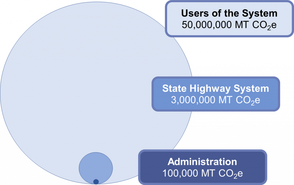
- Washington State DOT project-level GHG guidance (Washington State DOT 2018) provides that a quantitative analysis may be conducted at the planning level and referenced in the NEPA documentation. In the agency’s experience, GHG emissions from a single project action are usually very small (and projects often reduce GHG emissions). However, overall, users of the transportation system contribute close to half of the state’s GHG emissions. The agency believes that transportation GHG emissions are better addressed at the regional, state, and transportation systems level where multiple projects can be analyzed in aggregate.
Once plan-level effects are considered, the main issues to be considered at a project level are then:
- Whether the project is consistent with an adopted plan and associated environmental review that has considered GHG emissions.
- Whether some project alternatives are substantively more favorable or unfavorable than others in terms of GHG emissions or reductions.
- Whether additional GHG mitigation measures are warranted and appropriate.
4.1.2 Why Do Project-Level GHG Analysis?
Project-level GHG assessment includes consideration of project-specific GHG emissions effects in the design and selection of a preferred transportation project alternative and in the environmental documentation for the project. Individual project decisions may affect the emissions associated with the construction and maintenance of the project as well as the longer-term operation of vehicles on the project facility. A project-specific GHG assessment may be done in addition to a plan-level assessment (if one has been conducted).
GHG analysis and mitigation assessment may be conducted as part of environmental review procedures required under NEPA or state environmental laws. Section 2.3 of this guide discusses federal guidance related to the consideration of GHG emissions in environmental review. Some states’ environmental laws and regulations, such as California, Massachusetts, New York, and Washington, also require consideration of GHG emissions in state-level environmental reviews. In addition to meeting any applicable environmental review requirements, some state departments of transportation (DOTs) may include GHG consideration at the project level as part of state or departmental climate change policy issued by the Governor or Secretary/Commissioner or in response to public or stakeholder interest.
Key questions related to GHG emissions that may be addressed at a project level include:
- The type of project proposed to address a transportation problem. The Purpose and Need statement of an environmental review document describes the problem being addressed and why this particular project concept is being proposed as a solution. The initial definition of the project concept may be informed by systems-level decisions, such as whether to emphasize capacity expansion, multimodal, and/or “fix it first” solutions, that may have implications for GHG emissions.
- The project alternative(s) that are defined and evaluated. Many projects are relatively limited in scale/scope (e.g., road resurfacing or reconstruction) and may include only one project concept or alternative, which may be compared to the “no-build” option of not undertaking the project at all. Major projects may include multiple alternatives, such as highway expansion, transit expansion, intelligent transportation systems, or travel demand management, which can be evaluated and compared for GHG emissions impacts, among other criteria. Even single-alternative projects, however, can include choices that affect GHG emissions. For example, does a resurfacing project restore travel lanes as they are, or is the roadway restriped to provide bicycle lanes, which may help encourage mode shift?
- The specific elements and design details of each alternative. For example, will expanded bus service be provided by diesel or electric buses? What types of bicycle and pedestrian facilities will be included, given right-of-way constraints and local travel needs?
- Construction materials and activities unique to the project. For example, can demolition of an existing structure recover materials for reuse or recycling? Can a bridge project reuse beams from another project? How can construction be staged to minimize travel disruptions and detours?
Consideration of these issues at a project level does not necessarily require quantitative project-level GHG analysis. Choices may be made consistent with a general understanding of the expected GHG effects of each choice, with rationale documented in qualitative terms (which may include reference to planning-level studies or assessments). However, quantitative assessment may be useful in some situations to help inform and document the impacts of specific choices in more detail.
Tier 1 vs. Tier 2 Analysis
For major projects, a Tier 1 Environmental Impact Statement (EIS) may be conducted prior to developing a Tier 2 EIS. The Tier 1 step is a broad, programmatic analysis of the environmental consequences of alternatives. It is followed by more detailed Tier 2 environmental reviews focused on specific projects and improvements.
Given the conceptual nature of the Tier 1 alternatives, the level of detail in GHG emissions may be different than for a Tier 2 EIS. For example, modal traffic forecasts may be available at the Tier 1 level based on the general characteristics of each alternative (e.g., time and cost changes); however, detailed information on traffic operations effects (e.g., speed and delay changes at intersections) may not be available. Also, the information available to inform estimates of construction and maintenance emissions will be even more general and approximate (e.g., lane miles of new roadway) than in the Tier 2 stage (where specific details such as types and quantities of materials may still not be known until the final design is completed).
The limited detail that may be available at the Tier 1 level should not deter the agency from considering GHG emissions at this stage. On the contrary, some of the most important decisions affecting potential GHG emissions may be considered at the Tier 1 level. Examples include which modal options are considered and the general alignment and performance characteristics of a project. Waiting until Tier 2 will miss the opportunity to consider the GHG implications of these important choices.
4.1.3 Options for Plan-Level or Programmatic GHG Analysis
While the interim 2023 CEQ guidance (CEQ 2023a) states that a programmatic analysis may be referenced in project-level environmental documentation, no federal guidance is currently provided on what such a programmatic analysis should include or specific methods that should be applied. States are just beginning to provide examples of how a programmatic analysis might be conducted and what it might look like. The experiences of two states that have developed programmatic GHG information specifically to inform NEPA – Texas and Virginia – are described below.
Texas
Texas DOT (TxDOT) developed a statewide on-road GHG emissions analysis that provides an analysis of available data regarding statewide GHG emissions and on-road and fuel-cycle GHG emissions (Texas DOT 2018). TxDOT’s goal was to provide reasonably available information regarding climate change to the public and to provide information for consideration during the environmental analysis of a project.
TxDOT used the U.S. Environmental Protection Agency (EPA) Motor Vehicle Emissions Simulator (MOVES) model to estimate on-road GHG emissions from mobile sources for a base year of 2010 through a design year of 2040. Since TxDOT does not have a statewide travel demand model, a vehicle-miles traveled (VMT) estimate was projected based on population projections, historical traffic count data, and Texas county-specific fleet data. VMT was projected to increase at a linear rate from about 250 billion in 2010 to over 370 billion in 2040. Fuel-cycle emissions were estimated by multiplying statewide annual emissions by a factor of 27 percent, as cited per the EPA. The analysis noted that technology improvements were projected to reduce emissions more than VMT would increase them, with some uncertainty regarding future technology developments such as further fuel efficiency improvements and electrification.
TxDOT’s analysis does not provide an estimate of future year statewide “build” vs. “no-build” emissions, but it does provide a baseline emissions forecast for comparison.
Virginia
Virginia DOT (VDOT) developed a programmatic statewide GHG analysis that compared 2015 emissions to 2040 “no-build” and 2040 “build” emissions from surface transportation sources in Virginia, including on-road emissions as well as passenger and freight rail (Virginia DOT 2022a). The 2040 no-build scenario represents the transportation system as it exists in 2015, but with forecasted levels of population and job growth and corresponding travel volumes. The 2040 build scenario includes all modeled roadway projects represented in the long-range plans of the state’s metropolitan planning organizations (MPOs), as well as those in VDOT’s Six-Year Improvement Plan, and programmed and planned transit and rail projects that are reasonably expected to be funded over this time horizon. Both the 2040 no-build and build scenarios also consider levels of light-duty vehicle (LDV) and transit bus electrification consistent with state policies, including the adoption in 2021 of the Advanced Clean Cars rule. The statewide analysis also estimated construction and maintenance emissions as well as upstream (fuel-cycle) emissions.
VDOT developed this information to provide a resource for addressing GHGs in NEPA documents consistent with CEQ guidance. VDOT also developed template text describing the statewide analysis that is meant to be used when a project is determined to warrant quantitative GHG consideration but not a project-level quantitative GHG analysis, per agency guidance (Virginia DOT 2022a). VDOT specifies that this text be used if the project “was included in or otherwise consistent with the set of projects analyzed in the most recent statewide plan-year build/no-build GHG analysis.” The text notes that
The GHG effects of the statewide Build scenario compared to the No-Build were found to be small (0.3 percent increase), which is much less than the forecast 47 percent decrease in GHG emissions between 2015 and 2040 that is expected to occur as a result of ongoing fleet turnover to cleaner and more fuel-efficient vehicles despite ever-increasing vehicle-miles-travelled (VMT).
Virgina DOT (2022a)
And furthermore, that,
…on balance, all statewide highway capacity expansion projects were collectively found to cause a very small decrease in direct GHG emissions (0.03 percent), which is well within the margin of error in forecasts. Construction and maintenance emissions associated with the projects would increase overall emissions by less than 0.4 percent. The effect of this individual project would be expected to be much less than the collective effects of all planned statewide projects.
Virginia DOT (2022a)
The statewide GHG analysis is intended to streamline VDOT’s environmental assessment by avoiding the need for a project-specific GHG analysis in cases where the scale of the project and its GHG effects are too small to warrant extensive analysis effort. While the statewide analysis was conducted using state-of-the-practice tools and methods, a number of limitations are noted in the agency’s report, including:
- Limited ability to capture induced demand, including indirect impacts associated with land use change. VDOT’s report notes that land use effects related to highway or transit capacity expansion are generally speculative, localized, and difficult to model accurately and are therefore not captured in most of the travel demand modeling systems in use today, including VDOT’s statewide model.
- Limited ability of the model to estimate changes in congestion and speed. The statewide model does not explicitly model peak-period traffic, as many regional travel demand models do, and instead considers only a “congested” and a “free-flow” speed on each link.
- Limited ability to capture mode-shift effects, as the statewide model does not include transit or non-motorized modes. Mode-shift effects specific to transit and rail investments were estimated using a variety of project-specific methods, generally based on average emissions per passenger-mile or ton-mile, rather than a detailed evaluation of service levels and mode shifting. Mode-shift effects related to pedestrian and bicycle improvements or travel demand management strategies also were not modeled.
- Limited ability to capture the effects of traffic operations and other smaller-scale improvements due to the statewide scale and link-based network representation of the model.
- Construction and maintenance emissions are based on general, planning-level emissions factors rather than a detailed inventory of materials and fuel requirements.
- Carbon sequestration effects (e.g., loss of carbon sinks due to clearing of vegetation) are not considered.
These limitations are likely to be common to most DOTs with state-of-the-practice models and analysis methods.
Other Potential Approaches
To serve as a relevant programmatic reference in project-level environmental documentation, the project being studied should be included in, or at least consistent with (in type, scale, and scope) the set of projects or policies included in the programmatic evaluation. This would help ensure that the programmatic assessment reflects the emissions effects of the project.
A number of states have developed climate action plans or GHG reduction plans. These plans typically evaluate general sets of policies and/or investment programs that are intended to reduce emissions. In addition to the many climate action plans developed by state executive or environmental agencies, state DOTs in California, Maryland, and Oregon are known to have developed transportation-specific GHG reduction plans or strategies. To the extent that a proposed project is consistent with the policies or investments tested in one of these plans (e.g., investment in transit expansion or traffic flow improvements), information from the plan could potentially be cited in the project’s environmental documentation. However, many climate action plans specify policies or strategies only at a general level, and it may or may not be practical to link specific projects with high-level policies or strategies. The review conducted for this guide did not identify examples where this has been done.
Plan-level GHG assessments have been more commonly performed at the metropolitan level (often by MPOs)—sometimes as part of the Long-Range Transportation Plan (LRTP) process and sometimes as part of independent strategic assessments or climate plans. For example, California’s MPOs have completed Sustainable Communities Strategies analyses to demonstrate compliance with GHG reduction targets consistent with Senate Bill 375. Other MPO examples include the Portland, Oregon Metro Climate Smart Strategy (2015) and the Metropolitan Washington 2030 Climate and Energy Action Plan (2020). These assessments compare emissions under one or more long-range plan alternatives with the no-build alternative. Plan-level assessments made at the metropolitan level could potentially be cited in project-level environmental documentation for a project that is included in (or generally consistent with) an adopted MPO long-range plan that has been evaluated for GHG emissions effects. Again, the review conducted for this guide did not identify examples where this has been done.
Programmatic GHG assessments could also be conducted for groups of similar projects. For example, the FTA prepared a programmatic assessment for transit projects. FTA prepared the assessment to report on whether certain types of proposed transit projects merit detailed analysis of their GHG emissions at the project level and to be a source of data and analysis for FTA and its grantees to reference in future environmental documents for projects in which detailed, project-level GHG analysis is not vital. The assessment notes that “In cases in which project characteristics and assumptions are similar to those analyzed here, transit agencies considering BRT [bus rapid transit], streetcar, light rail, commuter rail, and heavy rail projects may incorporate this programmatic assessment by reference into their NEPA analyses” (FTA 2017).
Some state DOTs, including Colorado, Minnesota, and Virginia, have developed template text and standard analysis reporting tables or charts. These templates can be helpful in both streamlining the assessment effort and providing consistency across documents – both in cases where a project-specific analysis is required, and where reference is made to a programmatic assessment. Limited (if any) customization may be needed for Categorical Exclusion (CE) and simpler environmental assessment (EA) projects. For projects with potentially greater impacts, such as multi-alternative EISs, more customization may be required of descriptive text, especially if quantitative analysis is conducted.
4.1.4 Options for Project-Level GHG Analysis
If a GHG assessment is included in the environmental review, project alternatives are typically evaluated for their impact on emissions, and these impacts are described in the environmental documents for the project. A mitigation assessment may also be included. The selection of a preferred alternative can then include consideration of the findings from the GHG analysis. Options for GHG assessment include:
- No analysis due to expected minimal impacts. For example, the CEQ guidance does not specify that GHG analysis should be undertaken for CE projects, and states that have GHG guidance typically exclude most or all CEs from any requirement to consider GHG effects (CEQ 2023a).
- Reference to a statewide/programmatic analysis. If the DOT has conducted a programmatic or plan-level analysis, or if a relevant metropolitan or regional level analysis exists, documentation may reference this analysis rather than describing a project-specific evaluation. This approach could be suitable for projects that were included in the programmatic analysis or are of a nature similar to those projects and for which the programmatic analysis provides results representative of the project type.
- Qualitative, project-specific discussion. The DOT may describe the expected GHG effects of the project (direction and general magnitude) based on a general understanding of the effects of similar projects, and the various mechanisms by which the project is expected to affect emissions. These effects may include GHG-beneficial effects, such as smoothing traffic flow or encouraging mode shift out of vehicles, as well as GHG-negative effects, such as inducing more vehicle travel or more dispersed land use patterns. In some cases, a project may have effects working in opposite directions, and it may be impossible to state qualitatively whether the overall effect should be beneficial or harmful.
- Quantitative, project-specific analysis. The DOT may conduct a quantitative analysis to estimate the net GHG effects from traffic flow changes, mode shifts, technology changes, construction activities, etc. Even if a quantitative analysis is conducted, there are often limitations in the underlying data and models that result in uncertainties as to the expected GHG impacts. Known uncertainties should be disclosed, especially if they could affect the overall direction of GHG impacts.
States that have developed written guidance on considering GHG emissions in environmental review vary in which approaches are specified. States generally do not require any GHG consideration for CE projects due to expected small effects. For EISs and EAs, some states specify only a qualitative assessment, while others require a quantitative assessment for some or all projects.
4.2 GHG Emissions Sources to Include
A GHG analysis at any level may include some or all of the following emissions sources:
- Operational (direct, or tailpipe) emissions of vehicles using the facility or network once the project (or program of projects) is completed and open for use by the public. This source typically represents the majority of emissions and is nearly always included.
- Upstream or “fuel-cycle” emissions associated with the fuels or energy used by vehicles using the transportation network. These may include emissions from electricity generation, as well as emissions associated with the production and transportation of liquid or gaseous fuels and their feedstocks.
- Emissions associated with the construction of the study project alternative (or the set of projects included in a programmatic assessment), including emissions from construction vehicle activity and embedded (or “embodied”) emissions in materials used, and potentially emissions associated with changes in traffic patterns during the construction period.
- Emissions associated with operation and maintenance over the timeframe of the project or program – for example, resurfacing, removal of snow and debris, electricity for lighting, and vegetation management.
- Indirect emissions associated with secondary effects related to network changes, such as changes in land use resulting in changes in land cover and travel patterns. These are difficult to estimate with any reliability and are rarely quantified in practice. The Fiscal Responsibility Act of 2023 makes clear that environmental analysis of the project should be limited to the reasonably foreseeable environmental effects of the project.[1]
Sidebar 4-2: Emissions Scope Definitions
GHG analysts can encounter a confusing array of terminologies when it comes to defining scopes and sources of GHG emissions. Table 4-1 illustrates the potential relationships between the various sources of GHG emissions and CEQ’s definition of “direct” and “indirect” effects.
Table 4-1. GHG Emissions Sources Crosswalk
| Source | Direct Effects | Indirect Effects |
| Vehicles using the transportation system | “Tailpipe” emissions from vehicles using the project facility or traveling in the study area under current and projected conditions. |
|
| Construction and maintenance vehicles | “Tailpipe” emissions from vehicles being used to construct or maintain the project facility |
|
| Materials | On-site production of asphalt |
|
| Facility operations | Emissions from on-site power generation at project facilities (e.g., natural gas combustion or diesel generators at a rest area or rail station). |
|
| Other GHG sources and sinks (avoidance or removals) | Emissions released from disturbance of soil related to construction activities. |
|
In addition to the distinction between “direct” and “indirect” effects, the terms “scope 1”, “scope 2”, and “scope 3” emissions are widely used to characterize emissions in GHG accounting for inventory development. In the context of city or community-scale inventories these scopes are defined as follows:
- Scope 1 includes emissions that physically occur within a municipality or that are directly controlled by a particular organization at the site of their operations or facility.
- Scope 2 includes emissions that occur from the use of electricity, steam, and/or heating/cooling supplied or imported to the municipality or organization.
- Scope 3 includes those that occur outside the municipality or entity but are driven by activities taking place within the municipality’s or organization’s boundaries.
These scopes are not defined specifically in the context of a transportation project, but could be considered by analogy. “Direct effects” listed in the above table could correspond to scope 1 emissions. “Indirect effects” could include both scope 2 and 3 emissions, with scope 2 including electricity used by vehicles and facilities as well as other heating/cooling to serve project facilities, and scope 3 including upstream fuel-cycle emissions and embodied emissions in materials.
Consideration of upstream emissions for conventional fuels (gasoline and diesel) increases direct emissions by a relatively consistent amount, typically adding 20 to 30 percent, and is unlikely to affect the relative emissions differences among the alternatives. As electric or other alternative fuel vehicles make up an increasing share of the vehicle fleet, upstream emissions will increase in their relative importance. Project alternatives that include fuel technology differences (e.g., diesel vs. natural gas vs. electric buses or rail) should include upstream emissions if these differences are to be accurately evaluated. Emissions associated with a DOT’s annual construction and maintenance activities are estimated to be relatively modest compared to overall transportation system user emissions, on the order of 5 to 6 percent for a typical state’s highway system (Figure 4‑1). In some cases, however, differences in construction and maintenance emissions between project alternatives may be significant compared to differences in operational emissions for the same alternatives. For example, an analysis of a hypothetical major multimodal project in Virginia estimated a one-time impact of 34,000 metric tons of CO2e from construction of a highway widening and over 600 tons in additional annual maintenance emissions for the highway, compared to a net change in direct emissions of 900 tons for a bus alternative in 2045 (Virginia DOT 2022b). Construction emissions may be especially significant for energy-intensive processes such as tunnelling or constructing elevated facilities, as compared with provision of the same number of lane miles or track miles on the surface.
Source: Cambridge Systematics Inc. et al. (2022) based on data from multiple states.
A sample comparison of traffic-generated emissions with construction and maintenance emissions, calculated using the FHWA Infrastructure Carbon Estimator (ICE) tool, for various types of projects is shown in Table 4‑2. Note that these emissions can vary widely depending on factors such as the terrain and the materials and construction processes used, factors that are not typically captured in planning-level analyses like those provided by the FHWA ICE tool.
Table 4-2. Sample Emissions Estimates per Project Unit
| Project Description | Emissions (MT CO2e) |
| One lane mile of traffic (Annual average daily traffic of 20,000 over 25-year analysis horizon, at current vehicle efficiencies) | 91,058 |
| New roadway – Interstate/urban expressway (one lane mile) | 722 |
| Construction of additional lane (one lane mile) | 687 |
| Resurfacing (one lane mile) | 820 |
| Rehabilitation (one lane mile) | 2,172 |
| Construction of new bridge (two-span, one lane) | 127 |
| New BRT lane or right-of-way (one lane mile) | 484 |
| New light rail construction (at grade)—one track mile | 689 |
| New light rail construction (elevated)—one track mile | 5,966 |
| New light rail construction (underground soft rock)—one track mile | 172,414 |
| Surface parking (one spot) | 0.1 |
| Structured parking (one spot) | 7 |
| Off-street bicycle/pedestrian path construction—one mile | 54 |
| On-street bicycle lane construction—one lane mile | 54 |
| On-street sidewalk construction—one mile | 18 |
Source: Analysis using FHWA ICE v2.0 (Virginia DOT 2022a).
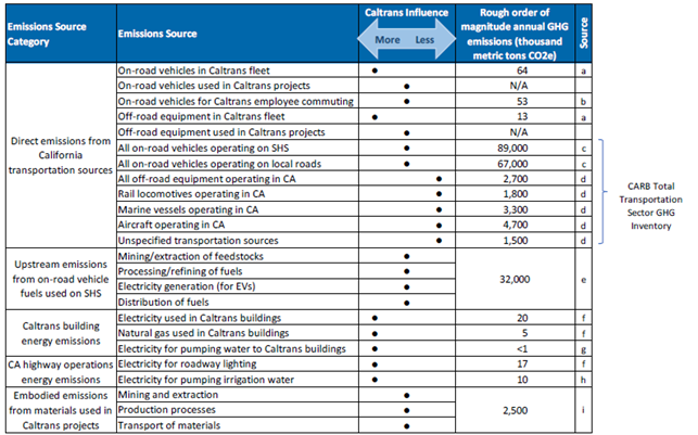
Table 4‑3 provides a sample of Virginia’s estimate of the relative contribution of the various direct and indirect emissions sources. Construction and maintenance make a relatively higher contribution in 2040 than in 2015 (around 4 percent vs. 2 percent) because on-road emissions are lower due to vehicle efficiency improvements and electrification, while construction and maintenance emissions are simply averaged over the entire 2015-2040 period with no accounting for future reductions in the carbon intensity of construction materials or vehicle operations. Table 4‑4 shows California’s estimates. Caltrans estimated that embodied emissions from construction materials were 2.5 million metric tons in 2017 or just under 3 percent of emissions from vehicle travel on the state highway system; another 0.12 MMT were measured in the agency’s internal operations (ICF 2020).
Table 4-3. Virginia Statewide GHG Inventory: Summary of GHG Emissions (Percent) by Source and Mode
| Source and Mode | 2015 | 2040 No-Build | 2040 Build |
| On-road Mobile Sources—Direct and Electricity Generation Emissions | 78.0% | 77.2% | 76.8% |
| On-road Transit Buses*—Direct and Electricity Generation Emissions | 0.2% | 0.1% | 0.1% |
| Urban Heavy Rail and Light Rail—Direct and Electricity Generation Emissions | 0.1% | 0.1% | 0.1% |
| Intercity Passenger Rail—Direct and Electricity Generation Emissions | 0.1% | 0.2% | 0.3% |
| Freight Rail—Direct and Electricity Generation Emissions | 1.1% | 2.1% | 2.2% |
| Subtotal, Direct + Electricity | 79.4% | 79.6% | 79.3% |
| Construction and Maintenance | 2.0% | 3.8% | 4.1% |
| Subtotal, Including Construction and Maintenance | 81.4% | 83.4% | 83.5% |
| Upstream Fuel Emissions (gasoline, diesel, compressed natural gas) | 18.6% | 16.6% | 16.5% |
| Total Including Upstream, Construction, and Maintenance | 100.0% | 100.0% | 100.0% |
* “On-road transit buses” includes buses operated by public transportation agencies. It does not include buses operated by private transit operators (such as intercity or coach services) or school buses. On-road transit buses are not included in the “on-road mobile sources” line.
Source: Virginia DOT (2022a)
Table 4-4. California Transportation Emissions Sources
Source: ICF (2020)
4.3 Tools and Methods for Planning-Level GHG Analysis
While the tools, methods, and data sources for plan-level GHG analysis often are the same as for project-level GHG analysis, there are some differences in which tools and methods will be most suited for each level of analysis. This section discusses plan-level/programmatic analysis tools and methods, and then Section 4.4 discusses project-level tools and methods, referring to (rather than duplicating) the plan-level discussion where appropriate.
4.3.1 Direct (Operating) Emissions
A plan-level analysis of GHG emissions, conducted for a state or a region, is likely to inherently include a GHG inventory (i.e., an assessment of current emissions from the transportation system) and baseline forecast (i.e., future projected emissions with adopted policies and programs, but without additional proposed actions). Often, the same tools can be used for evaluating plan-level GHG emissions effects as for developing GHG inventories and baseline forecasts. If the state DOT has a travel demand model and specific projects are modeled as part of the statewide plan or program evaluation, the model may be used to develop plan- or program-level forecasts. An MPO will generally be able to use its model to evaluate long-range plan or Transportation Improvement Program (TIP) alternatives. If the agency has the capacity to apply the EPA MOVES emission factor model [or Emissions Factor (EMFAC) in California], MOVES can be used in conjunction with data generated by the travel demand model. Otherwise, VMT outputs can be used in conjunction with fuel efficiency estimates by vehicle type and carbon content factors to estimate GHG emissions.
For agencies without a travel demand model, VMT may need to be projected based on growth trends, and “off-model” methods can be used to estimate plan impacts. GHG-specific tools may also be used, such as the VisionEval open-source model or the FHWA Energy and Emissions Reduction Policy Analysis Tool (EERPAT). “Off-model” methods are also likely to be needed to evaluate the emissions effects of any types of projects that are not evaluated well by the statewide or regional model. For example, if the model does not include a transit, walk, or bike mode choice component, it will not provide information on the effects of these modal investments or mode-shifting policies. Even models that do include these modes may not be sensitive to the effects of smaller projects. Examples of “off-model” methods include project calculators, such as the FHWA Congestion Mitigation and Air Quality Improvement (CMAQ) Calculator Toolkit and Cal-B/C, and customized spreadsheet-based calculations using data such as elasticities and empirical results observed from other projects. See Appendix B for additional information on these tools.
Table 4‑5 provides sample illustrations of how CO2 emissions can be easily calculated based on VMT, fuel efficiency, and carbon content factors. More information on systems-level analysis tools and methods can be found in NCHRP WebResource 1: Reducing Greenhouse Gas Emissions: A Guide for State DOTs (Cambridge Systematics et al. 2022).
Table 4-5. Illustration of CO2 Emissions Estimates from VMT
| Vehicle type | Vehicle-miles of travel (millions) | / Miles per gallon (2025) | Multiplied by carbon content (kg CO2/gal) | = CO2 emissions (tons) |
| Light-duty vehicles | 2,979 | 25.9 | 8.78 | 1,013,000 |
| Medium trucks | 73 | 8.7 | 10.21 | 86,000 |
| Heavy trucks | 246 | 6.4 | 10.21 | 393,000 |
| All on-road vehicles | 3,314 | 1,514,000 | ||
| Data Source | Travel demand model | U.S. DOE – AEO 2022 Reference Case | U.S. EPA (2021b) | Calculation |
Notes: Carbon content assumes 100 percent gasoline for LDVs and 100 percent diesel for heavy trucks and buses. The carbon content for emissions from medium trucks is also for diesel fuel, assuming that average MPG in the Annual Energy Outlook is expressed in MPG diesel equivalent.
Any travel activity modeling system will have limitations when it comes to providing data to estimate GHG emissions and changes in these emissions. Each agency should be aware of both the capabilities and limitations of their own modeling platform. In particular, any limitations that could substantially affect the magnitude or even the direction of estimated GHG effects of plan alternatives should be disclosed. Common limitations of travel demand models, particularly those developed for statewide applications, include: estimating only daily traffic rather than peak-period volumes and traffic conditions; not including a mode-choice component; using simplistic methods to estimate truck traffic; low geographic resolution; and inability to capture the effects of relatively small projects.
4.3.2 Upstream Emissions
Data and tools to estimate upstream emissions include:
- The U.S. EPA Motor Vehicle Emissions Simulator (MOVES). While MOVES itself does not estimate upstream emissions, it can estimate the energy directly consumed by vehicles in their operation, and this energy consumption can then be used as an input for other tools that estimate the emissions associated with fuel and electricity production.
- The Argonne National Laboratory Greenhouse Gases, Regulated Emissions, and Energy Use in Technologies (GREET) model. GREET can provide fuel-cycle emission factors (multipliers) for gasoline, diesel, and natural gas, and many other fuels. The model includes default settings relevant to the United States as a whole but may be customized considering numerous fuel production pathways. Table 4‑6 shows sample emission factors for passenger cars in 2025 using GREET1_2022 with the default fuel production pathways.
- The U.S. EPA eGRID database. The database provides recent-year GHG emission factors for electricity generation regions and states in the U.S. Since the GHG intensity of electricity generation can vary widely across the nation, the analyst should look up factors for the appropriate region or state. For future year analyses, the analyst may need to consider projections for changes in GHG intensity based on the latest adopted or proposed state policies and/or utility plans. The state environmental or energy agency can often assist with this. See Sidebar 4-3 for guidance on using eGRID data.
Sidebar 4-3: Using eGRID Data to Estimate EV Emissions
- Visit https://www.epa.gov/egrid/download-data and download the latest eGRID data [as of this writing, eGRID2022 (xlsx)].
- Find your state (ST) or subregion (SRL) and look up the “U.S. annual CO2 equivalent combustion output emission rate (lb/MWh).”
- The average rate for the United States in 2020 is 1,319 lb CO2e per megawatt-hour (MWh) = 1.319 lb per kilowatt-hour (kWh) × 0.454 kg/lb = 0.60 kg CO2e/kWh.
- Estimate the average energy consumption of an EV in kWh per mile. The following are examples of how to make such estimates:
- Take the average MPG of a vehicle (25.9 for LDVs projected in 2025, from the 2022 Annual Energy Outlook Reference Case), convert it to mi/kWh by dividing it by the energy content of the fuel in kWh/gal, and then multiply by an energy efficiency ratio (EER) reflecting the higher efficiency of electric drive (e.g., 3.0), and then convert to kWh/mi. In this example: 25.9 mi/gal · 33.4 kWh/gal = 0.775 mi/kWh × 3.0 EER = 2.33 mi/kWh = 0.430 kWh/mi or 43 kWh/100 miles
- kWh/gal sourced from Wikipedia. Note that estimates of kWh/gal vary slightly depending upon the assumed energy content (heating value) of the fuel.
- Average energy consumption for electric LDVs can also be sourced from U.S. EPA or other industry ratings of kWh/100 miles. Further assumptions may be needed to estimate a fleet-weighted average. This method also assumes that the fleet of EVs currently being sold is representative of relative efficiencies in future years.
- Multiply the energy consumption rate (in kWh/mi) by the emission factor per unit energy (in kg/kWh) to get the emission factor per vehicle-mile. In this example, 0.430 kWh/mi × 0.60 kg/kWh = 0.258 kg CO2e/mi.
- A similar approach can be applied to medium and heavy-duty EVs and electric buses. Since diesel fuel has approximately 11 percent higher energy content per gallon than gasoline, the equivalent conversion factor would be 37.1 kWh/gal.
Note: MWh = megawatt-hour; kWh = kilowatt-hour
Table 4-6. GREET Emission Factors by Fuel Type, Passenger Cars, 2021
| Fuel Type | Direct (Vehicle Operation) GHG Emissions (g/mi) | Upstream (Feedstock + Fuel) GHG Emissions (g/mi) | Life-cycle GHG Emissions (g/mi) | Life-cycle Emissions as a percentage of Gasoline Vehicle Emissions | Upstream Emissions as a percentage of Direct Emissions |
| Gasoline | 330 | 72 | 402 | 100% | 22% |
| Diesel (CIDI, conventional diesel) | 284 | 59 | 343 | 85% | 21% |
| Diesel (CIDI, soybean-based B20) | 284 | 17 | 301 | 75% | 6% |
| Compressed natural gas | 273 | 82 | 355 | 88% | 30% |
| Plug-in hybrid electric (U.S. electricity mix) | 102 | 134 | 236 | 59% | 131% |
| Electric vehicle (U.S. electricity mix) | 0 | 175 | 175 | 44% | NA |
Source: Argonne National Laboratory, GREET1_2022. (See Appendix B for more details.) CIDI = Compression ignition direct injection; B20 = 20% biodiesel blend to diesel fuel; g/mi= grams of CO2e/mile.
The California Air Resources Board (CARB 2022) also publishes tables of estimated life-cycle carbon intensities for numerous fuel types and production pathways certified under the state’s low-carbon fuel standard. A figure published by CARB shows the intensity ranges of various fuels adjusted for energy efficiency ratio (EER), the relative efficiency at which the vehicle uses fuel compared to a conventionally fueled vehicle. This represents the grams of CO2e emitted per megajoule of conventional fuel displaced. CARB values may differ from GREET values as a result of differences in assumptions about production pathways and also about the treatment of life-cycle effects, such as indirect land use change associated with crop biomass and leakage of natural gas.
4.3.3 Construction and Maintenance Emissions
Emissions related to the construction and maintenance of a project include:
- Carbon emissions associated with energy, fuel, and industrial processes in the production and transport of materials used (e.g., CO2 from calcination of limestone used in cement). These are known as “embedded” or “embodied” emissions.
- Emissions from construction and maintenance vehicles and activities. Maintenance emissions may include snow removal, vegetation management, sweeping, pavement maintenance, striping, litter pickup, and other roadway and bridge deck repair and maintenance.
- Emissions changes related to traffic changes during the construction period (e.g., lane reduction, detours).
One recent study estimated that nearly half of construction and maintenance emissions are related to fuels used by vehicles, while most of the remainder are embodied emissions in paving materials (Figure 4-2).
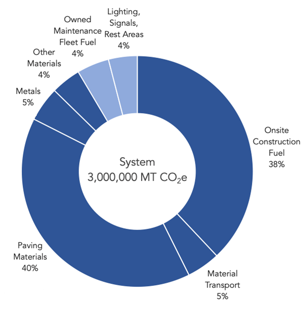
Source: Cambridge Systematics et al. (2022) based on data from multiple states.
Note: Emissions that are primarily from construction are shown in darker blue, while emissions that are primarily from maintenance are shown in lighter blue; however, for some categories, construction and maintenance cannot be clearly separated.
For statewide or programmatic application, as well as for application early in project development, a relatively simple tool is needed that only requires basic planning-level inputs such as lane miles of roadway, rail, or bridge construction. The FHWA ICE tool accepts these relatively simple inputs and is used by a number of states for planning and/or project-level applications. Other tools may be required for a more detailed evaluation of project designs, materials, and mitigation measures.
4.4 Tools and Methods for Project-Level GHG Analysis
When GHG emissions are to be quantified, agencies generally balance best practice technical methods with data availability and level of effort. For example, GHG analyses are typically done using travel data and emissions analysis methods already developed for traffic and air quality analyses. Quantification of construction and maintenance emissions may require a GHG-specific tool and basic data collection to support that tool, and estimates for transit and rail modes (if included) may require some custom data sources and methods. Additional information on GHG analysis tools is found in Appendix B of this guide, as well as in other documents such as NCHRP WebResource 1: Reducing Greenhouse Gas Emissions: A Guide for State DOTs (Cambridge Systematics, Inc. 2022) and Oregon DOT (2018b). Early consultation between agencies or functional areas can ensure that the most appropriate models and assumptions are used and that GHG methods are consistent with the data and methods for traffic and air quality analysis.
4.4.1 Direct (Operating) Emissions
Most environmental documents for which a quantitative GHG analysis will be required are also likely to include an air quality analysis that addresses one or more other air pollutants, including particulate matter, carbon monoxide (CO), and/or mobile source air toxics (MSATs). Many of the same tools and data sources that are used for other pollutants can also be used for GHG analysis. For example, if MOVES is already being used, expanding the analysis to include GHGs may be as simple as checking another box for desired outputs. Some states, including Minnesota and Virginia, specify that the same methods be used for GHG analysis as for MSAT analysis if an MSAT analysis is conducted. If an MSAT analysis is not conducted, Minnesota specifies that the Minnesota Infrastructure Carbon Estimator (MICE) tool, which requires only daily VMT and average speed, can be used. Analysts can look for synergies between the GHG and air quality analysis to minimize the additional effort required to include GHG emissions.
Quantification of direct (tailpipe) GHG emissions effects requires 1) quantification of any changes in travel (VMT, transit service, speeds); 2) determination of emissions per VMT based on vehicle technology; and 3) application of emission rates to travel changes. Travel changes are typically estimated using one set of models or methods, with another set of methods to estimate emission rates. In some cases, a single tool may cover both travel activity and emissions data. The following sections discuss common methods for identifying travel activity changes and emissions rates and then discuss some specific topics including the use of the MOVES model, data and methods for transit and rail emissions, and accounting for EVs.
Travel Activity
Methods available for estimating project-level travel activity changes may include the following:
- A regional or statewide travel demand model, which can be used to evaluate major (i.e., capacity expansion or transit investment) projects. These models may be able to evaluate changes in traffic speeds related to changes in travel patterns and VMT as long as the project has large enough effects. However, in many cases, it is likely that changes in travel patterns due to the project are too small to measurably affect speeds and congestion on either the project facility or other study area roads—i.e., the effect is lost within the “noise” of the model. In such cases the model should still be useful for estimating baseline traffic volumes and speeds on the project facility. It may also be useful for evaluating mode shift as long as it has a mode choice component. Regional models, if available, are usually preferred over statewide models since regional models usually have greater spatial resolution and are more likely to have mode choice and peak-period components.
- A refined sub-area model (including travel demand or microsimulation models), which may have been developed to improve traffic and/or transit ridership estimates in specific major corridor studies. These are generally labor-intensive to develop and would not be developed specifically for GHG estimation but they can be used for that purpose if they are available.
- Highway Capacity Manual or similar resources or methods for estimating speed changes from capacity and operational improvements on specific roadways. These methods are suited for estimating speed changes but not volume changes since trip generation and distribution effects are not captured. The methods may be applied to capture emissions effects of changes in delays on cross-streets on the project links as well as the project links themselves, but will not capture larger study area effects resulting from changes in traffic patterns.
- Project-specific evaluation tools such as FHWA’s Congestion Mitigation and Air Quality (CMAQ) Improvement Program Emissions Toolkit, CMAQ calculators developed by the state DOT or an MPO, and Cal-B/C. These tools accept relatively simple inputs, such as number of lanes and average daily traffic volumes, and are likely to be able to estimate GHG emissions changes directly.
- Transit-specific tools such as the FTA Simplified Trips-on-Project Software (STOPS) model or the Florida DOT Transit Boardings Estimation Tool (TBEST) to estimate changes in transit ridership.
- Simplified estimates using data from similar projects or services. Examples include using the same average ridership for new transit service as is seen on existing service or estimating speed changes for traffic operations improvements based on speed changes observed for similar projects.
- Analysis of service plans, to estimate emissions associated with bus and rail transit vehicles (e.g., the number of train or bus trips per week multiplied by the route length, multiplied by the number of vehicles per train). Deadheading should be considered in addition to planned baseline vehicle revenue-miles (VRM) and changes in VRM for various project alternatives.
Emission Rates
Methods available for estimating emission rates include the following:
- Direct application of the MOVES model. This is generally most appropriate for larger projects where a travel demand model is being used. To expedite the use of MOVES for multiple projects, templates or postprocessors may be set up to translate changes in traffic data (speeds and volumes by roadway link) into MOVES inputs such as speed distributions and VMT. Further discussion of the use of MOVES for project GHG analysis is provided below.
- Application of VMT-based emission factors from MOVES analysis (grams per vehicle-mile) conducted for a programmatic GHG assessment or another project. Average emission factors can be applied to changes in VMT for each alternative without considering the effects of speed changes. Alternatively, some agencies have run MOVES to establish lookup tables of emission factors by speed, which can be applied to changes in the estimated speeds for the project roadway.
- Application of fuel-based GHG emission factors to VMT and fuel/energy consumption (miles per gallon or kWh/mile) by fuel type. This is necessary for vehicle types not modeled in MOVES, including locomotives, electric buses, and potentially vehicles using other clean fuels.
In general, the level of effort required for the GHG analysis is expected to be commensurate with the level of effort applied to evaluate other project impacts for environmental documentation and/or project planning purposes, such as changes in VMT, congestion, transit service levels, and transit ridership or mode share. This suggests that the same tools that are applied for other analyses can provide the foundation of the GHG analysis for the project in question.
MOVES Setups
The EPA has published two documents directly relevant to using MOVES for GHG analysis, in addition to general documentation such as the MOVES user guide. The documents are not written specifically for project-level GHG analysis to support environmental documentation but can inform the use of MOVES for such analysis. EPA also discusses various topics on its “MOVES and Related Models” website.
- Using MOVES for Estimating State and Local Inventories of Onroad Greenhouse Gas Emissions and Energy Consumption (EPA 2016) describes approaches for developing an on-road GHG inventory and the implications of each of these approaches. It discusses the data input options that are most important for estimating on-road GHG emissions and explores which inputs should be populated with locally derived data versus data from the MOVES default database to improve the quality of the results. The document also describes how MOVES can be used for scenario planning and policy efficacy analysis for travel efficiency and vehicle and fuel technology strategies.
- Greenhouse Gas and Energy Consumption Rates for Onroad Vehicles in MOVES3 (EPA 2020) is a technical document that provides information that may serve as useful background for the specific assumptions embedded in MOVES, such as the federal light- and heavy-duty vehicle fuel efficiency and GHG emissions standards that are included in the model.[2] MOVES is updated on a regular basis, but the latest version of MOVES (and any associated documentation) may lag the latest adopted federal standards. Users should be aware of any discrepancies and note those discrepancies when reporting MOVES-generated emissions outputs. The main effect for environmental documentation purposes will be on absolute horizon year emissions; the percent difference between horizon year emissions among alternatives should be less affected.
Pollutants: If MOVES is already being used for modeling project-level air quality impacts, it is a relatively simple matter to include GHG emissions. This can be done by adding CO2e (Pollutant 98) to the panel of pollutants to be output. Using CO2e instead of CO2 captures the effects of other greenhouse gases, such as methane (CH4) and nitrous oxide (N2O), in addition to CO2, and reports them in CO2-equivalents.
Processes: GHG emissions are associated with starts, running emissions, and extended idling (for heavy trucks). However, it is typical in a project evaluation context to only consider running emissions, which are expressed on a grams per mile basis. This is because a typical roadway project is assumed to affect only the activity of a vehicle that occurs over a trip (distance driven, speeds) and not the number of vehicle trips that are taken. In some cases, such as a multimodal project, it may also be appropriate to consider reductions in cold start emissions associated with trips that are entirely mode-shifted from automobiles to another mode. However, the improved accuracy of doing so should be weighed against the added resource requirements.
Time span: One important difference between GHG and air pollutant analysis is that only annual GHG emissions will be of interest, whereas some air pollutants may need to be reported for peak hour periods. To reduce run time, MOVES can generate an annual GHG inventory by estimating hourly emissions individually and summing them to produce the year’s emissions, known as “pre-aggregating” data. However, pre-aggregation can lose some of the non-linear effects of temperature. EPA (2016) discusses further when and how it may be most appropriate to aggregate GHG data over time spans.
Analysis domain: An important choice facing the analyst is whether to apply MOVES at the county domain, project domain, or a custom domain (e.g., multi-county or state, using county inputs). The required inputs vary significantly between the county and project domain scales. If MOVES is already being used for one type of domain for air pollution analysis, the same domain may be used for GHG analysis. If the user faces a choice, the scale of the project should be considered. If the project can be defined using just one or a small number of network links, the effort required should not differ substantially. However, for a large project requiring many links (and potentially including other “affected links” on the network), the resource requirements to develop inputs and run MOVES at the project domain can be much greater than using the county domain (see Sidebar 4-4), since inputs must be provided for every link, rather than in aggregate format for the analysis network. This is one reason why FHWA recommends using MOVES at the county domain scale for MSAT analysis. If the project extends into more than one county, using data inputs (e.g., age distributions, inspection and maintenance programs, fuels) for a “representative” county is likely to provide sufficient accuracy with less effort than providing discreet sets of inputs for multiple counties.
Definition of study area/affected links: Even when using MOVES at the county domain scale, it is not necessary to model changes on all roads in the county or counties being studied. The travel data analysis may be restricted to output data (e.g., VMT, speed distributions) for just a set of “affected links” with volumes and speed changes exceeding a certain threshold. For example, FHWA (2016b) suggests MSAT analysis thresholds such as a ± 5% to 10% or more change in annual average daily traffic depending upon the level of service and a change of ± 10% or more in travel time or intersection delay. This requires first doing a travel analysis of the entire study area to identify the “affected links” to be included in the emissions analysis. If more than one alternative is to be evaluated, some links may meet the criteria for some alternatives but not others. The “affected links” can be defined based on the alternative for which the greatest changes are anticipated and used as a consistent set of links for all alternatives to facilitate apples-to-apples comparisons; or a separate no-build vs. build comparison can be made for each alternative.
Sidebar 4-4: Comparison of MOVES County and Project Domains for a Large Highway Corridor Project
The Virginia DOT compared using MOVES3 at the project domain vs. county domain for evaluation of a hypothetical highway widening project along a 36-mile segment of I-95. The analysis considered affected links (based on the FHWA MSAT criteria) in a five-mile buffer of the highway. Compared to the county domain estimates, the project domain application resulted in emissions estimates about 10 percent higher, possibly due to the consideration of grade effects (steeper grades increase emissions compared to flat terrain). However, these differences were consistent across alternatives, meaning that the two methods showed very similar relative effects (percent changes) between alternatives. VDOT concluded that the project domain application did not provide significant additional useful information for comparing project alternatives. The agency also found that the project domain application was considerably more time-intensive than the county domain application.
Source: Virginia DOT (2022b)Transit and Rail Emissions Data Sources and Methods
Changes in public transportation service levels (bus or rail) and/or freight rail proposed as part of a project may result in changes in GHG emissions from those services, as well as displaced GHG emissions from reduced automobile traffic. Sources of data to support changes in emissions related to transit and rail include the following.
Public transportation service levels: Baseline public transportation vehicle activity in the project corridor and any proposed changes in activity may be estimated considering current and proposed operating plans, including train and bus schedules and/or General Transit Feed Specification data on existing services. For rail services, the analyst should be sure to differentiate between vehicle-miles and train-miles, where vehicle-miles is equal to the sum of train-miles multiplied by the vehicles per train (including locomotives and passenger-carrying cars).
Rail and public transportation emission rates (grams GHG per vehicle-mile). Potential sources include:
- The MOVES model (buses only). MOVES produces emissions data for three types of buses: intercity buses (source type 41), transit buses (source type 42), and school buses (source type 43). Emission rates can be estimated by dividing total emissions by VMT. If only an aggregate VMT estimate for buses is available, use vehicle type 40 (bus) for Motor Bus and Commuter Bus (MB, CB). MOVES provides forecast year as well as base year emission rates.
- National Transit Database (NTD) data on fuel use by type of fuel and VMT by mode type and fuel type. NTD data may be used to estimate fuel consumption per vehicle-mile or train-mile for base year services.
- Fuel emission factors. A source such as The Climate Registry can be used to estimate emission factors for CO2 and other GHGs per gallon, to apply to estimate of energy consumption measured in gallons of fuel consumed, such as estimated from the NTD. Sample fuel emission factors per gallon are shown in Table 4‑7.
Table 4-7. Fuel Emission Factors per Gallon
| Fuel Type | Units in NTD Reporting | Emission Factor: CO2 (kg/gal) | Emission Factor: N2O(g/mi) | Emission Factor: CH4 (g/mi) | Comments |
| Gasoline | Gallons | 8.78 | 0.0082 | 0.0085 | Gasoline Medium and Heavy Duty Vehicles (Trucks and Buses), EPA Tier 2 |
| Diesel | Gallons | 10.21 | 0.0048 | 0.0048 | |
| Biodiesel | Gallons | 9.45 | 0.002 | 0.002 | |
| Natural Gas | Gallons of diesel equivalent | 7.349 | 0.001 | 10.000 |
Source: The Climate Registry (2020), Tables 2.1, 2.4. Natural gas rate of 0.05444 kg/standard cubic foot (scf) converted at a rate of 135 scf/gallon diesel equivalent, from BAF Technologies, “CNG 101,” citing compressed natural gas industry standard.
- Annual Energy Outlook (AEO) projects modal energy intensities. The AEO is updated annually by the U.S. Department of Energy and includes a number of useful data tables through an interactive data browser. Transportation Table 7: Transportation Sector Key Indicators and Delivered Energy Consumption provides estimates of energy intensity for light-duty stock and freight trucks (miles per gallon) and freight rail (ton-miles per thousand British thermal units or Btu). Other AEO tables provide more details on vehicle stock, activity, and energy consumption by mode and technology, such as stock and energy consumption estimates for medium vs. heavy trucks. Base-year efficiencies may be adjusted by the ratio of forecast-year to base-year efficiency for the most similar mode from the AEO, per the example shown in Table 4‑8. For example, buses are not included in the AEO but are subject to the same medium- and heavy-duty fuel economy standards as trucks.
Table 4-8. Projected Average Modal Energy Intensities
| Mode | Units | 2021 | 2030 | 2040 | 2050 |
| Light-duty (stock) | Miles per gallon (gasoline) | 24.2 | 27.7 | 29.7 | 30.5 |
| Freight Truck | Miles per gallon (diesel) | 7.3 | 8.4 | 9.5 | 10.0 |
| Rail | Ton-miles per thousand Btu | 3.5 | 3.7 | 4.0 | 4.2 |
Source: Annual Energy Outlook, 2022 Reference Case
- Oak Ridge National Laboratory Transportation Energy Data Book (TEDB) energy intensities per passenger-mile or per ton-mile. The TEDB is updated annually with the latest available national estimates of energy intensity per passenger-mile or ton-mile. These estimates may be used in cases where (for example) a ridership forecast or freight tonnage forecast is available, but actual service levels are not known. Application of the average rate assumes average ridership, utilization, and/or other factors consistent with the U.S. average for a similar service and does not take project or corridor-specific conditions into account. Table 4‑9 shows an example where base year energy intensities from TEDB are projected to a forecast year using modal energy intensity projections from AEO. In this example, the AEO projects that the energy efficiency of freight rail per ton-mile will increase by 16 percent between 2017 and 2040. The example assumes that this efficiency improvement applies to both passenger and freight rail and that GHG intensity is proportionate to energy intensity (i.e., no change in fuel sources or the carbon intensity of these sources).
Table 4-9. Average Rail Energy Intensities per Passenger-Mile or Ton-Mile
| Mode | Units | Energy Intensity (Btu/unit): 2015 | Energy Intensity (Btu/unit): 2040 | CO2 Intensity (kg CO2/unit): 2015 | CO2 Intensity (kg CO2/unit): 2040 |
| Passenger Rail | Per passenger-mile | 1,644 | 1,381 | 0.132 | 0.111 |
| Freight Rail | Per ton-mile | 293 | 246 | 0.023 | 0.019 |
Sources: Energy intensity—National average for commuter rail or freight rail, from Oak Ridge National Laboratory Transportation Energy Data Book, Edition 38.1. Converted to CO2 intensity at a rate of 10.21 kg CO2 per gallon (The Climate Registry 2020) and 127,371 Btu per gallon (Energy Information Administration). 2040 vs. 2015 efficiency improvement of 16 percent based on AEO projections.
- Alternative Fuels Data Center (AFDC). The AFDC publishes a variety of information related to fuel use and efficiency, generally from secondary sources. For example, Figure 4‑3 shows average fuel economy by major vehicle category.
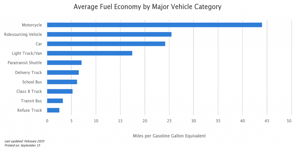
Source: AFDC (2020) as gathered from various sources.
- Displaced automobile emissions. The APTA Recommended Practice: Quantifying Greenhouse Gas Emissions from Transit (APTA 2018) identifies two sources of displaced emissions: transportation efficiency (mode shift, or avoided car trips) and land use efficiency (leading to shorter trips, more walk/bike trips, and lower rates of car ownership). Note that the original (2009) version of the APTA recommended practice also identified congestion relief effects. Congestion effects are omitted from the 2018 practice due to the lack of data for the measurement of congestion benefits and the lack of agreement in the academic literature about whether public transportation reduces congestion.
- Transportation efficiency or mode shift. If a multimodal travel demand model is used to forecast project travel changes and ridership, it may be possible to estimate mode-shift effects directly from that model by comparing automobile VMT with and without the project alternative. Projects that cause a relatively small change in VMT relative to total VMT in the model area, however, may not accurately register in the VMT output of a network model, which is likely to fluctuate between model runs due to “noise” in the network assignment process. It may be more accurate to estimate reductions in automobile travel using an estimated increase in transit trips (derived from the model’s mode choice component or from other methods) combined with two key parameters – trip length and the “prior drive mode share” of new transit riders (i.e., the share of new riders who previously drove a vehicle). These parameters might be estimated from model data, surveys of existing transit riders, or literature sources if no local data is available.
- Land use efficiency. APTA provides information from Transit Cooperative Research Program (TCRP) research to quantify the secondary emissions benefits resulting from land use effects of existing and new transit service (McGraw 2021). The land use multiplier is based on a statistical analysis of the relationship between transit investment/service and land use patterns to estimate the long-term effects of transit in terms of reducing the need for auto travel through more efficient land use patterns that result in trips that are shorter and/or feasible by walking or bicycling. The referenced TCRP report notes that the most appropriate multiplier can vary substantially based on the type of service and its urban context, with the greatest effect for fixed-guideway services in larger and/or denser metropolitan areas.
Sidebar 4-5: Emissions Effects of Rail and Public Transportation Projects: Example
A statewide GHG analysis for VDOT (Virginia DOT 2022a) compared the GHG emissions effects of a statewide 2040 “build” vs. “no-build” program. The build program included 12 BRT and passenger rail projects and five freight rail projects, as well as bus service increases based on local operator transit development plans. The results, shown in Table 4-10, illustrate the relative magnitude of various emissions sources. The total reduction in emissions was estimated to be 9,392 tons, or 0.04 percent of the total projected 27.2 million metric tons of statewide direct and fuel-cycle transportation emissions in 2040. This reflects the relatively small contribution of transit and rail to total statewide transportation emissions (91,000 tons from transit buses and passenger rail and 570,000 tons from freight rail in 2040) and also the limited incremental impact that projects are likely to have within the context of a widely built out transportation system.
Table 4-10. Net Effects of Modal Projects (Statewide Example)
| Project | Net GHG Change in metric tons |
| Emissions from new bus service | 7,929 |
| Displaced auto emissions from new bus service: mode shift | (3,484) |
| Displaced auto emissions from new bus service: land use effects | (7,937) |
| Displaced auto emissions from new bus service: congestion relief effects | (10) |
| Emissions from new light and heavy rail service | 2,219 |
| Displaced auto emissions from new light and heavy rail service | (4,338) |
| Emissions from new commuter and intercity passenger rail service | 31,528 |
| Displaced auto emissions from new commuter and intercity passenger rail service | (28,719) |
| Emissions from new freight rail service | 2,718 |
| Displaced truck emissions from new freight rail service | (9,299) |
| Total, Transit and Rail Build Projects | (9,392) |
Accounting for Electric and Fuel-Cell Vehicles
Older versions of MOVES (including MOVES3) did not directly estimate GHG emissions effects associated with electric or fuel-cell vehicles. Common workarounds included entering an EV fraction of LDVs by model year and adjusting MOVES output to reduce emissions in proportion to the fraction of VMT driven by EVs in the forecasted calendar year. MOVES4, released in 2023, provided improved capabilities to model EVs. MOVES4 includes forecasts of default national EV fleet fractions and also provides an Alternate Vehicle and Fuel Technology Tool, allowing users to enter local EV fractions. MOVES4 also includes the capability to model heavy-duty battery EVs and fuel-cell vehicles. The calculation of energy and emissions assumes EVs have no tailpipe emissions and does not include upstream emissions associated with electricity generation.
Because of the time it takes for the fleet to turn over, some years can elapse before EV sales targets translate into similar electrification levels for the on-road vehicle fleet. For example, an aggressive policy scenario for the Carbon Free Boston study estimated that 40 percent of new LDV sales would be electric in 2030, approaching 80 percent in 2040 (Cambridge Systematics, Inc. 2019). However, the fraction of light-duty VMT electrified would not reach 40 percent until 2038 and 80 percent until after 2050 (Figure 4‑4). The VMT fraction slightly leads the population fraction since new vehicles are driven more miles per year than older vehicles. This analysis also assumes that EVs are driven the same number of miles per year as conventional fuel vehicles.
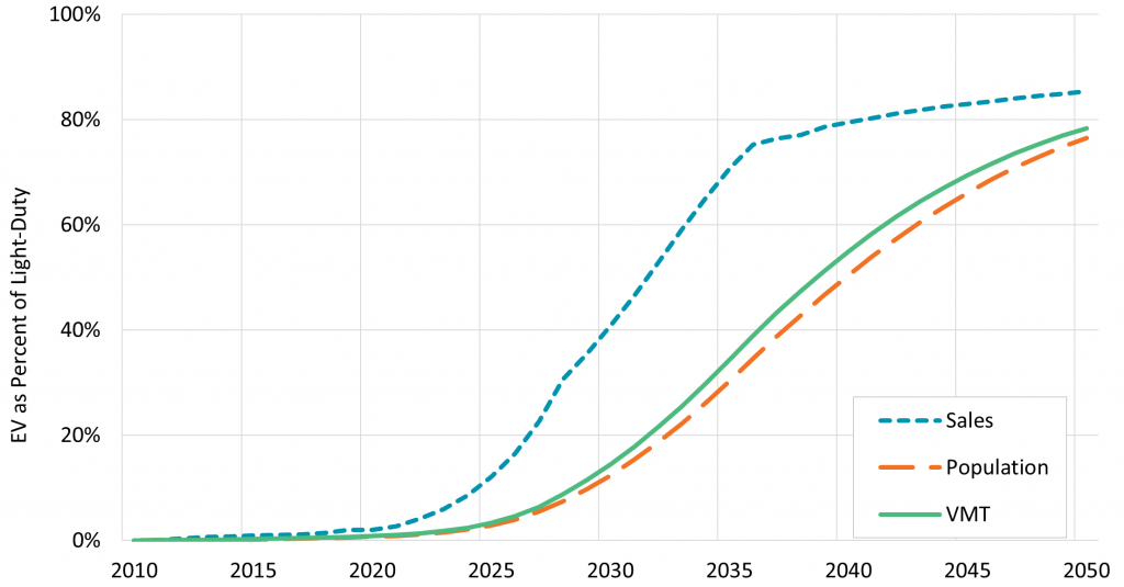
Figure 4‑4. Sample Comparison of EV Sales, Population, and VMT Fractions
Source: Cambridge Systematics (2019)
When using emission rate data from sources other than MOVES, such as the AEO, the analyst should be aware of what assumptions (if any) are built into the data regarding electrification of zero-emission vehicles. AEO provides tables showing fuel efficiency projections by vehicle and technology type. To adjust for the effects of a different level of zero emission vehicles than assumed in the AEO reference forecasts, use the MPG estimates for gasoline or diesel vehicles from the AEO to estimate fuel consumption, then apply a carbon content factor per unit of fuel as illustrated above in Table 4-6, and then reduce emissions in proportion to the share of zero-emission vehicles.
4.4.2 Upstream Emissions
The same data and tools can be used to estimate upstream emissions at a project level as at a programmatic level, as described in Section 4.3. These are most likely to be the GREET model for upstream emission factors and the EPA eGRID database for electricity emissions.
4.4.3 Construction and Maintenance Emissions
A number of tools are available to assist with estimating construction and maintenance emissions at a project level, mainly focusing on embodied emissions associated with materials, as well as construction vehicle activity. An overview of tools is provided in Appendix B, and a more extensive list and review are provided in NCHRP WebResource 1: Reducing Greenhouse Gas Emissions: A Guide for State DOTs (Cambridge Systematics, 2022). Some of the most relevant include:
- The FHWA ICE tool, a relatively simple tool that requires basic planning-level inputs such as lane miles of roadway, rail, or bridge construction.
- The FHWA Life Cycle Assessment for Pavement (LCA-Pave) tool, which can provide a more detailed analysis of the life-cycle effects of specific pavement options.
- GreenDOT, which includes both materials and equipment with more detailed input requirements than ICE.
- Environmental Product Declarations which disclose emissions associated with specific material sources. The agency may need to build up GHG estimates from disclosed carbon contents and material volumes if they are using non-standard materials that are not reflected in the tool(s) they are using.
Information on specific materials and quantities may not be known at the time the environmental documentation is developed, which is typically prior to the final design stage. However, an agency may decide to use a lower-carbon material or construction method, either as part of their standard specifications, or as part of project-specific mitigation. Information on the relative carbon emissions of that material or method compared to conventional materials and methods could be documented as part of the environmental documentation.
If information is available on expected traffic changes during the construction period, such as lane reduction and detours, GHG effects could be forecast using simulation models (e.g., lane closures) or sketch methods (e.g., comparison of original and detour length routes, traffic volumes, emissions per vehicle-mile). GHG emissions from temporary traffic changes are usually not forecast in practice due to a lack of readily available data, but they might be considered for a project with significant construction-period traffic impacts, especially if a construction-period air quality analysis is already being conducted. If forecasts are unavailable, qualitative statements could still be made about planned efforts to reduce GHG emissions associated with lane closures and/or detours (e.g., by scheduling lane closures during off-peak periods). Table 4‑11 compares these tools for evaluating construction and maintenance emissions based on data requirements and project types suited for analysis. For a more detailed evaluation and comparison of these and other tools, see Appendix B.
Table 4-11. Comparison of Tools for Construction and Maintenance Emissions
| Tool | Input Data Requirements | Project Type(s) |
| FHWA ICE |
|
|
| FHWA Life Cycle Assessment for Pavement (LCA-Pave) |
|
|
| GreenDOT |
|
|
| Environmental Product Declarations |
|
|
4.5 Equity Considerations
Equity is considered in environmental review according to federal requirements and guidance outlined in Section 3.2, which outlines requirements to identify and address the disproportionately high adverse human health and environmental effects of federal programs, policies, and activities on low-income and minority populations. Section 5.4 of this guide provides additional resources on outreach and engagement of equity-focus communities.
Unlike other regulated pollutants such as particulate matter, volatile organic compounds, and oxides of nitrogen (NOx), GHGs do not cause direct localized health impacts. Where the GHGs are emitted does not matter, only the total quantity. Therefore, the only equity issues directly related to GHG emissions are community scale and global equity concerns related to the effects of climate change. However, GHG emissions are often correlated with other air pollutant emissions that do have localized effects and strategies that reduce GHG emissions typically reduce other pollutants as well. Therefore, community members may not perceive an important distinction between GHGs and other air pollution when it comes to equity. Project developers should be sensitive to community concerns generally related to poor air quality and to consideration of project design and mitigation strategies that can improve local air quality while also reducing GHG emissions.
4.6 Communicating Findings and Drawing Conclusions
The environmental documentation should clearly communicate the methods used in assessing GHG emissions, and the findings of any GHG assessment that is conducted, whether qualitative, quantitative, or referencing a programmatic assessment. For a quantitative analysis in particular, the findings may be summarized in the main text with additional detail in a technical appendix, which may be the same appendix providing details for other air quality analyses.
4.6.1 Qualitative Assessments
A qualitative project-level GHG assessment should describe the ways in which the project is expected to affect GHG emissions as well as the degree to which the project’s design and potential effects on GHG emissions are consistent with any regional or statewide climate action plans, policies and/or goals and objectives. The qualitative assessment may also reference any programmatic actions the agency or state has undertaken to reduce transportation GHG emissions. A sample outline of a qualitative GHG assessment is shown in Sidebar 4-6.
Sidebar 4-6: Sample Outline: Project GHG Report (Qualitative)
1. Introduction a. Brief description of the project and its purpose and need. b. Brief description of alternatives, including no-build.
2. Climate Change a. Brief description of the greenhouse effect, greenhouse gases, and global warming potentials. b. Statewide GHG emission inventory—total transportation GHG emissions and transportation as a percentage of total state emissions. c. State and/or regional actions with regard to GHG emission reductions, if any (e.g., GHG reduction policies, goals, targets, and/or climate action plans, including any specific to the transportation sector).
3. Project Setting* a. Brief description of the expected effect of the project alternatives on traffic variables that may affect GHG emissions, such as volumes, speeds, congestion, transit ridership, vehicle fleet mix, induced travel demand, etc. b. GHG reducing considerations in project design.
4. Analysis Outcome a. Findings of any statewide or regional programmatic GHG analysis that has been conducted and that the project is consistent with. b. A summary of whether the completion of the project is expected to result in less or more GHG emissions from vehicles operating on the facility. c. A discussion of GHG emissions from the construction of the project. To the extent known, this could include a description of the equipment and fuels that will be used, the duration of the construction and how it may be staged, and the duration and location of any detours resulting from the construction of the project. d. A discussion of GHG emissions from maintaining the facility once the project is completed. To the extent known, this could include a general description of what the maintenance activities could be, how far into the future they may occur, the equipment and fuels that may be used, etc. e. A description of how the project aligns with any statewide or regional GHG plans or policies.
5. Conclusion a. An overall conclusion regarding the project, the preferred alternative, and the impact on GHG emissions.
* Typically, a GHG emissions analysis is included within an Air Quality Section of an environmental document or an Air Quality Report or Appendix. If so, these items may already be prepared and need not be duplicated. If climate change will be considered in a separate section of an environmental document or report/appendix, it is suggested these items be included.
4.6.2 Quantitative Assessments
A quantitative project-level assessment should describe the ways in which the project is expected to affect GHG emissions, as well as the degree to which the project’s design and potential effects on GHG emissions are consistent with any regional or statewide climate action plans, policies, and/or goals and objectives. The quantitative assessment should describe the key data sources, methods, and assumptions for the GHG analysis, as well as the findings of the quantitative analysis. The assessment should describe any potential GHG effects that could not be modeled or for which uncertainties may affect the findings. The assessment may also reference any programmatic actions the agency or state has undertaken to reduce transportation GHG emissions. A sample outline of a quantitative GHG assessment is shown in Sidebar 4-7.
Sidebar 4-7: Sample Outline: Project GHG Report (Quantitative Analysis)
1. Introduction a. Brief description of project and its purpose and need. b. Brief description of alternatives, including No-Build.
2. Climate Change a. Brief description of the greenhouse effect, greenhouse gases, and global warming potentials. b. Statewide GHG emission inventory – total transportation GHG emissions and transportation as a percentage of total state emissions. c. State and/or regional actions with regard to greenhouse gas emission reductions, if any (e.g., GHG reduction policies, goals, targets, and/or climate action plans, including any specific to the transportation sector).
3. Project Setting* a. Brief description of the expected effect of the project alternatives effect on various traffic variables that may affect GHG emissions, such as volumes, speeds, congestion, transit ridership, vehicle fleet mix, induced travel demand, etc. b. GHG reducing considerations in project design.
4. Technical Approach a. Are upstream emissions included? i. If yes, model(s) used b. Brief description of the scale and scope of the traffic network used in the analysis. i. Same network as MSAT analysis, if MSAT analysis is also performed c. Models used for operational emissions i. Traffic model/methodology ii. Emission model d. Selection of Analysis Years e. Construction/Maintenance emissions i. Scale and scope of the traffic network and community to be included ii. To the extent known, provide a description of the equipment and fuels that will be used, the duration of the construction and how it may be staged, and duration and location of any detours resulting from the construction of the project. iii. To the extent known, description of what the maintenance activities could be, how far into the future they may occur, the equipment and fuels that may be used, etc. The results of the emissions from maintenance of the facility can be displayed.
5. Analysis Outcome a. Emissions analysis i. Operational emissions are summarized by alternative, including upstream emissions if included. ii. Construction/maintenance emissions summarized by alternative. iii. Total project emissions summarized by alternative. b. A summary of whether the completion of the project is expected to result in less or more GHG emissions. c. A description of how the project aligns with any regional or statewide GHG analyses, plans, or policies. d. Mitigation measures considered and mitigation to be implemented, if any.
6. Conclusion a. An overall conclusion regarding the project, the preferred alternative, and the impact on GHG emissions.
* Typically, a GHG emissions analysis is included within an Air Quality Section of an environmental document or an Air Quality Report or Appendix. If so, these items may already be prepared and need not be duplicated. If climate change will be considered in a separate section of an environmental document or report/appendix, it is suggested these items be included.
4.6.3 Timeframe of Emissions Reporting
Environmental analyses are typically done considering a time horizon that includes a base year as well as a horizon (forecast) year 10 to 20 years after opening. In some cases, conditions in the opening year or an interim year may also be evaluated.
Additional timeframes may be warranted for reporting of GHG emissions. First, some states have set GHG emission reduction targets for specific years, e.g., 2030, 2035, or 2050. It may be desirable to report the effects on emissions in these years, to assist in identifying how projects may contribute to GHG emission reductions in those years in combination with other GHG reduction measures. While conducting underlying traffic analysis for additional years could require significant additional effort, a simplified approach that could be taken would be interpolating or extrapolating results from years that are already being modeled for project analysis purposes. Early coordination could also help align analysis years with desired GHG reporting timeframes, if such reporting is an important consideration.
Agencies may also wish to report cumulative GHG emissions across all years in the analysis period. (“Cumulative” in this context simply refers to emissions over a multi-year time horizon, rather than “cumulative effects” of actions as defined for NEPA purposes.) Reporting cumulative emissions can be advantageous for two reasons:
- Climate change is related to the accumulation of GHGs in the atmosphere over time, and therefore, reporting cumulative emissions provides a more complete picture of the project’s effects than just reporting annual emissions in one or two years.
- Reporting cumulative emissions provides a way to make direct comparisons between one-time construction-period emissions and ongoing emissions as viewed through the horizon year snapshot. This is especially helpful when emissions reductions from project operations may offset added emissions during construction. Otherwise, the analysis year reporting would either exclude construction-period reporting altogether or construction-period emissions could be annualized over the project lifetime to estimate an “annual” construction effect. A “payback” analysis could also be considered to evaluate the time it takes to offset the increase in construction emissions through reduced operating emissions (assuming the project reduces operating emissions).
Estimating cumulative emissions changes would ideally require year-by-year estimates of traffic changes and emission rates. However, doing so is likely to require a high level of effort as compared to the additional value of information obtained. Instead, simplified interpolation/extrapolation methods could be used to infer annual changes based on base year and horizon year forecasts.
4.6.4 Drawing Conclusions
Drawing conclusions regarding the importance of a project’s GHG emissions or climate change effects is one of the greatest challenges faced by project reviewers and analysts. Unlike for ambient air pollutants, which have concentration criteria established based on human health effects, GHG emissions contribute to local health problems only indirectly, through global climate change and its effects. It may therefore be tempting to compare the scale of project emissions (or the difference between project alternatives) to total statewide, national, and/or global emissions. However, CEQ (2023a) cautions against this (see Sidebar 4-8). Clearly, decreases in emissions, or small increases, are preferable to large increases, and large changes are worth extra effort to evaluate than small changes. However, there is no accepted standard or benchmark for defining “small” vs. “large” or for determining whether a given level of increase or decrease is acceptable.
Sidebar 4-8: CEQ Guidance on Comparisons with Global Emissions
The CEQ cautions against comparing the scale of project emissions to global emissions. According to their 2023 guidance:
The totality of climate change impacts is not attributable to any single action, but is exacerbated by a series of actions including actions taken pursuant to decisions of the Federal Government…. NEPA requires more than a statement that emissions from a proposed Federal action or its alternatives represent only a small fraction of global or domestic emissions. Such a statement merely notes the nature of the climate change challenge, and is not a useful basis for deciding whether or to what extent to consider climate change effects under NEPA. Moreover, such comparisons and fractions also are not an appropriate method for characterizing the extent of a proposed action’s and its alternatives’ contributions to climate change because this approach does not reveal anything beyond the nature of the climate change challenge itself—the fact that diverse individual sources of emissions each make a relatively small addition to global atmospheric GHG concentrations that collectively have a large effect.
CEQ (2023a)Some agencies have established minimum emissions thresholds to identify sources that should or should not be included in a regulatory framework or reporting system. For example, the U.S. EPA Greenhouse Gas Reporting Program sets 25,000 metric tons of GHG per year as the threshold for emissions reporting requirements; California and Washington have set the same threshold for sources regulated under each state’s cap-and-trade program. These thresholds are set to avoid an excessive level of effort directed at relatively small contributors; they are not meant to imply a level of significance to impacts, nor are they intended to apply to the evaluation of alternatives for transportation projects.
While a significance threshold for GHGs at a project level does not exist, in the end, the environmental document needs to support the decision made regarding the project. To that end, in its environmental review documents, the lead agency could provide a conclusory summary of the GHG assessment performed, substantive differences between the alternatives considered, measures that would be implemented to reduce emissions, and the project alternatives’ overall consistency with broader and long-term GHG emission reduction and sustainability goals. GHG effects may be considered in the decision as one effect among many potential benefits and impacts of the proposed project.
Applying a “social cost of carbon” could represent one approach towards comparing GHG effects against other project impacts that can be monetized, such as travel time savings, air pollution reductions, and crash reductions. However, many environmental impacts are not easy to monetize and environmental analysis documents are not typically presented as a cost-benefit analysis. The 2023 CEQ guidance recommends applying the social cost of carbon to GHG emissions effects of alternatives, although it notes that cost-benefit analysis is not required (CEQ 2023a).
4.6.5 Examples
In California, for projects that provide congestion relief or otherwise increase roadway capacity (including operational improvement projects that are expected to address future demand volumes), guidance calls for developing a quantitative analysis of GHG emissions using either the CT-EMFAC2014 or CT-EMFAC2017 model. Caltrans provides a sample table reporting format, as shown in Figure 4‑5.
Source: Caltrans (2020a)
Virginia DOT’s template text in its air quality resource document (Virginia DOT 2022a) suggests reporting emissions effects in three tables:
- A summary of emissions (metric tons CO2e) by alternative and source in the base and horizon years.
- The change in horizon year emissions compared to the No-Build by alternative and source.
- The percent change in horizon year emissions compared to the No-Build by alternative and scope of emissions included.
Sources are separated into direct sources, including on-road mobile, passenger rail, and commuter bus; maintenance emissions; upstream (fuel-cycle) emissions, including electricity; and construction impacts. Separating direct and upstream emissions provides for consistency with emissions inventories where different sectors (e.g., transportation, electricity) include only the sector’s direct emissions. Separating emissions by mode provides for greater transparency. An example reporting table is shown in Figure 4‑6.
Source: Virginia DOT (2022b)
VDOT also recommends reporting cumulative emissions. The template text suggests these can be estimated by estimating emissions in each year for each alternative. For the no-build alternative, a linear interpolation of annual emissions between the base and horizon years can be performed. For each build alternative, a start year needs to be assumed. Prior to the start year, emissions for the build alternative may be assumed to be the same as for the no-build. After the start year, direct, upstream, and maintenance emissions may be factored by the ratio of horizon year build to no-build emissions. Construction emissions can be spread evenly over the construction period preceding the opening year.
The I-5 Columbia River Crossing study conducted jointly by the Oregon and Washington State DOTs included a comparison of emissions changes, both absolute and proportional, at different scales—project-level, and regional, as shown in Figure 4‑7.
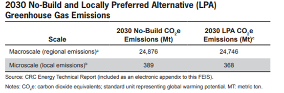
Source: Oregon DOT and Washington State DOT (2011)
There is no single “correct” geographic scale reporting emission changes. Regional-scale reporting typically shows a larger absolute reduction since all changes in emissions across the regional transportation network are considered, but a smaller proportional reduction since the change in emissions is measured relative to a much larger baseline. Project-level reporting more directly captures the changes occurring along the project facility itself. A study area that is larger than the project alignment (e.g., a buffer around a corridor or a set of “affected links” identified based on speed and volume changes per FHWA MSAT guidance) can represent a middle ground, capturing most of the project’s absolute impacts, but not overly diluting proportional changes.
Minnesota DOT also provides a standard reporting format for projects that affect traffic flow. The reporting specifies cumulative reporting of both operational and construction emissions, in addition to operational emissions for the base year, No Action and Build alternatives, and the difference between Build and No-Build (Figure 4‑8). For projects that do not affect traffic flow, only construction emissions are reported.
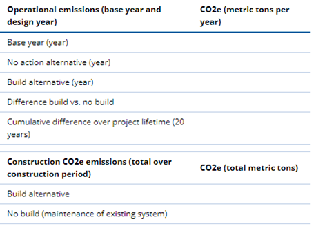
Source: Minnesota DOT (undated)
4.7 Mitigation Measures
One of the purposes of NEPA is to identify mitigation measures to improve environmental outcomes of proposed federal actions. NEPA regulations (40 CFR 1508.1) state that mitigation means “measures that avoid, minimize, or compensate for effects caused by a proposed action or alternatives as described in an environmental document or record of decision and that have a nexus to those effects.” The regulations further state that while NEPA requires consideration of mitigation, it does not mandate the form or adoption of any mitigation. The regulations state that mitigation includes:
- Avoiding the impact altogether by not taking a certain action or parts of an action.
- Minimizing impacts by limiting the degree or magnitude of the action and its implementation.
- Rectifying the impact by repairing, rehabilitating, or restoring the affected environment.
- Reducing or eliminating the impact over time by preservation and maintenance operations during the life of the action.
- Compensating for the impact by replacing or providing substitute resources or environments.
The CEQ’s 2023 interim guidance discusses mitigation of GHG emissions, and instructs agencies to evaluate the quality of mitigation to ensure that it is additional, verifiable, durable, enforceable, and will be implemented. An agency’s decision on a proposed action should identify the mitigation measures that the agency commits to take, recommends, or requires others to take. Monitoring intensity and duration should be aligned with the mitigation action taken. More general CEQ guidance on mitigation further discusses procedures to:
- Ensure that mitigation commitments are implemented.
- Monitor the effectiveness of mitigation commitments.
- Remedy failed mitigation.
- Involve the public in mitigation planning.[3]
In the sample of 21 EIS and EA documents reviewed for Appendix C, no examples were found in which GHG mitigation measures were proposed specifically with the aim of offsetting anticipated emissions increases between the build and no-build alternatives or in which the effects of specific measures identified as GHG “mitigation” were quantified. In some cases, the document made general statements that emissions could be reduced during the construction phase through traffic management planning and/or materials selection. Some documents noted that GHG emissions are projected to decrease between the base year and analysis year (due to technology improvements consistent with federal regulations) and that GHG increases between the build and no-build alternatives (if any) are expected to be small relative to that decrease.
Many of the documents reviewed did discuss either project-specific or programmatic actions that had been taken by the agency or the state to reduce GHG emissions, even if they were not identified specifically as “mitigation” measures for NEPA purposes. This included, for example:
- Noting that the agency and/or state already have various programs or strategies in place to reduce GHG emissions, either generally (unrelated to the project), or as a byproduct of other mitigation measures such as construction air quality. For example, the EA Georgia DOT produced for the I-285 & SR 400 Reconstruction Project (see Appendix C, column P) notes that Georgia is a member of the Climate Registry, a nationwide voluntary effort to quantify GHG emissions from all sources and lay the foundation for potential future carbon emissions trading and mitigation efforts; and that measures to minimize air quality impacts during construction would also aid in reducing GHG emissions. Reference may also be included to projects or strategies that are included in other planning documents such as long-range plans, corridor plans, modal plans, or congestion management plans (although inclusion in such plans does not guarantee the strategy or project will be implemented).
- Noting that mitigation measures are inherent in the selected project alternative. For example, the I-5 Columbia River Crossing EIS (see Appendix C, column D) notes that the locally preferred alternative inherently involves several mitigation measures, including providing bicycle and pedestrian infrastructure, providing transit options, implementing tolls, increasing efficiency of transportation systems, and supporting transit-oriented development.
Sidebar 4-9: Example — Reference to Programmatic GHG Reduction Activities
An EIS prepared by Maryland DOT (Maryland DOT 2022) provides an example of references to programmatic GHG emissions reduction activities.
- “Maryland is committed to reducing GHG and to preparing our State for the impacts of climate change. The Maryland Commission on Climate Change (MCCC) and its Mitigation Working Group (MWG) have demonstrated that commitment by working collaboratively with experts and stakeholders across State and local agencies, environmental, non-profit and academic institutions. The resulting body of work quantifies baseline GHG emissions by sector to understand the impacts that specific plans, policies, and programs will have on future emissions economy-wide. Statewide analyses do not indicate that the HOT lanes will impede Maryland’s ability to meet our GHG emission reduction goals. In fact, the Greenhouse Gas Reduction Act (GGRA) Plan documents Maryland’s existing and future emissions reductions under several scenarios, all of which include this project. The document illustrates that Maryland will not only meet the 40% by 2030 goal, but that we are dedicated to working together to exceed that goal and to strive for a 50% reduction by 2030.”
Based on NEPA’s 40 most asked questions, FHWA notes that “The mitigation of impacts must be considered whether or not the impacts are significant.”[4] It can therefore be considered good practice to include GHG emission reduction measures in the environmental review for a project, despite the lack of a significance threshold or determination.
Examples of GHG reduction measures that have been proposed as part of the design of a project alternative rather than specifically as mitigation measures include:
- Transit options.
- Bicycle and pedestrian accommodations/improvements.
- Geometric design and/or operations strategies to improve traffic flow.
- Long-term travel demand management (e.g., pricing, incentives, ridesharing, employer outreach programs) to reduce vehicle travel and peak-period congestion in the corridor.
Examples of other measures that might be referenced or proposed as GHG reduction measures, whether or not they are formally identified as “mitigation” for NEPA purposes, include:
- Use of low-carbon materials or construction techniques.
- Clean construction vehicles (which may already be noted as an air quality mitigation measure for some projects).
- Short-term travel demand management to reduce congestion and emissions impacts during construction.
- Carbon sequestration through vegetation planting and management.
- Purchase of carbon offsets.
Sidebar 4-10: Carbon Sequestration, Renewable Energy, and Offsets as GHG Mitigation Measures
Carbon Sequestration
Transportation agencies may identify opportunities to sequester carbon, either directly in the right-of-way (out of the clear zone) of a project, or at another location, as a strategy to mitigate GHG emissions related to a project. Examples of sequestration include tree planting and enhancing soil carbon through nutrient augmentation of existing vegetation. Sequestration projects, if done appropriately, can have valuable ecological and social benefits, including reducing the urban heat island effect, restoring habitat, mitigating air pollution and noise, holding moisture, and enhancing green space.
Agencies should understand that the scale of emissions that can be sequestered is likely to be small compared to the scale of emissions from the operation of vehicles on the project or even its construction. To ensure significant sequestration, the planting of the vegetated area will almost certainly go well beyond the project footprint. For example, a two-lane concrete bridge span of approximately 100 feet with roughly 20-foot-high piers in Portland, Oregon, requires about 18,700 trees or 400 trees per acre over 50 acres growing for 30 years. While all living vegetation sequesters carbon and provides environmental and aesthetic benefits, only trees have enough scale to be worth the effort in DOT properties (Proudfoot et al. 2015). Mature old growth trees sequester carbon at the fastest rate, while younger trees sequester carbon more slowly, at a rate of around 1 metric ton of GHGs per acre per year for younger fir trees.
The GHG mitigation benefits of sequestration can also depend upon a variety of factors with complex interactions, such as the type of vegetation, what it replaces, the condition and treatment of the soil, the climate, the overall integrity of the ecosystem, the analysis timeframe, and what happens with the site for decades to come. If a DOT wants to evaluate the carbon sequestration of tree planting, they must first consider the embodied emissions of producing the nursery stock as well as planting the material as a deficit, that later will “break even” on its carbon and eventually be a net removal of GHGs.
Renewable Energy Generation in the Right-of-Way
Transportation agencies have developed or considered uses of the right-of-way for renewable energy generation. This has the potential to generate revenue as well as produce clean energy to offset other GHG emissions, especially in areas where the electricity grid is powered by higher-emissions sources such as coal and natural gas. On-site solar and sometimes small vertical wind turbines can match the scale needed for lighting on a new facility but will have a small impact compared to system user emissions. As an example, Oregon DOT developed a solar facility in the right-of-way of an interchange between I-5 and I-205. This 107-kilowatt capacity system provides enough power in an hour to fully charge one large passenger EV.
While solar often displaces more emissions of GHGs and other pollutants from the power grid than a tree sequesters, the decision between solar panels and trees must be made carefully. In particular, deciduous trees may provide much-needed shade to a building and may do more good by displacing the emissions associated with generating power that would have been used for air conditioning. When the tree has lost its leaves in the colder months, the need for heat is decreased due to solar heat gain. In suitable locations, solar installations can be used as shade or wind block facilities for park-and-ride lots.
Carbon Offsets
Carbon offsets are an environmental commodity that is sold to negate another party’s emissions. Offsets may involve sequestration, or any number of other mitigation actions not related to the transportation project. The receiver of the money must “originate” a project that provides additional carbon avoidance or removals from a unique project anywhere in the world. Purchasing carbon offsets may be an option for mitigating GHG emissions, but it also has pitfalls and should not be considered a complete substitute for mitigation. Among other issues, offsets are likely to require a separate funding source as they may not be eligible for the federal and/or state funding sources used for the transportation project. Further, the range of prices on carbon offsets varies dramatically in the voluntary but verified markets. In many states, there is an established “social cost of carbon” which is the basis for their regulatory programs which can set the expectation that the project pays that price. Local stakeholders often desire local offset projects, but there may be limited local potential or costs may be prohibitive. Finally, there are questions about the extent to which offset actions are “additional” (i.e., generating real GHG reductions) or whether they would have happened even if they had not been purchased as offsets.
The Minnesota DOT’s Greenhouse Gas Analysis Process identifies several design and construction practices that can help reduce emissions from projects, most of which can be evaluated using the MICE tool:
- Full-depth reclamation.
- Cold in-place recycling and cold central plant recycling.
- Warm-mix asphalt.
- Recycled concrete aggregate.
- Increase in overall wetlands, tree cover, or planted area.
Tools that could potentially be used to evaluate and quantify the benefits of GHG reduction and mitigation strategies are listed in Appendix B. Examples include:
- Emission factor models such as MOVES and EMFAC.
- Project-level tools to evaluate travel reduction and/or traffic flow improvements, such as CMAQ emissions calculators.
- Tools for assessing clean vehicles (for construction and maintenance), such as the Alternative Fuel Life-Cycle Environmental and Economic Transportation (AFLEET) and the Diesel Emissions Quantifier.
- Tools for evaluating construction and maintenance emissions (such as ICE and LCA-Pave) that allow for the evaluation of alternative materials and/or construction practices that could reduce emissions. Emission factor models such as MOVES and EMFAC.
4.8 Project- or Program-Level GHG Assessment in Relation to GHG Goals or Targets
An increasing number of states are setting GHG reduction goals, targets, or requirements. As of 2022, half of all states had set a target either by statute, executive order, or both, according to the Center for Climate and Energy Solutions. These targets often aim to achieve deep emissions reductions (80 to 100 percent) by 2050, and often set aggressive interim year targets as well (e.g., 2030 or 2035). These goals or targets are generally economy-wide, although in some cases, they will be specified for the transportation sector. Targets may be set on a total or per-capita basis. Some regional agencies and municipalities are also setting goals or targets and tracking emissions. Agencies are also tracking emissions to measure progress against goals or targets. In December 2023, FHWA issued a Final Rule (88 FR 85364) to establish a national GHG emissions performance measure. States and MPOs are required to estimate GHG emissions on the National Highway System, starting with a base year of 2022, and to set declining targets, with the first report due in 2026 for a 2025 reporting year. As part of the Carbon Reduction Program established by the Infrastructure Investment and Jobs Act of 2021, FHWA also required each state to develop a Carbon Reduction Strategy that supports efforts to reduce transportation emissions and identifies projects and strategies to reduce these emissions. Strategies were due to FHWA in November 2023 and must be updated at least every four years.
A plan or programmatic-level GHG assessment of transportation projects will often include a projection of total emissions from surface transportation sources, or at least on-road mobile sources, comparing emissions for a base year and a forecast year for a build and no-build scenario. If a forecast year is selected consistent with a year in which the state has set goals or targets, the relative emission reductions resulting from the actions in the plan, as well as other policies incorporated in the baseline, can be compared against the goal or target reduction. The state goal or target may be expressed as a reduction from a different year (e.g., 2005, as compared to a 2020 study base year), but if the state has been tracking emissions by sector, the difference can also be compared against the goal or target baseline. If the study forecast year does not coincide with a target year, linear interpolation might be applied to provide a rough estimate of progress against targets.
If only a project-level GHG evaluation is conducted, the project will probably have a small effect relative to total statewide transportation GHG emissions. It can be stated that the greater the reduction in emissions from the project, the more likely the project is to support meeting targets. Conversely, if the project increases emissions, it is more likely to work at cross-purposes to achieving targets. Making any statements beyond this requires understanding the broader context of transportation system actions and anticipated emissions from the future system. For example, a project that individually increases emissions may still be part of an overall plan that is expected to decrease emissions.
4.9 Examples in Practice
The following section provides examples of how GHG effects have been evaluated and communicated in environmental documents for transportation projects. The examples are meant to illustrate the state of practice at the time this guide was developed. Since practice on this topic is rapidly evolving, readers should consider these examples as illustrative rather than as intended to be emulated and should carefully consider their own state’s requirements and needs when developing a state-specific approach.
A few states, including Minnesota DOT and Virginia DOT, as described below, have developed “template text” or standard language that can be inserted into environmental documents. These examples can serve as a guide to other state DOTs that are seeking to develop template language to include in environmental reviews for their agency. Other state DOTs could assess the examples, determine how they apply to their state and project conditions, and modify them as appropriate. Any template language should be applicable to their state’s greenhouse gas and climate change policies and requirements as well as to the project’s purpose and need and the alternatives under consideration. Careful thought should be applied to the use of template language in project environmental reviews to ensure that the project circumstances match those of the language of the template statement.
4.9.1 Minnesota DOT: Greenhouse Gas Analysis Standard Attachment for Categorical Exclusion Projects
Minnesota DOT provides a Word document with standard text and tables for reporting GHG effects for CE projects (Minnesota DOT 2020a, “Greenhouse Gas Analysis Standard Attachment for Categorical Exclusion Projects”). The attachment has different text and table formats (up to one page each) for projects that do not change traffic flow vs. those that do. For projects that do not change traffic flow, only construction CO2 emissions are discussed. For projects that change traffic flow, operational and construction emissions are discussed, with the following template provided for narrative text:
MnDOT evaluates greenhouse gas (GHG) emissions from projects due to concerns about current and future impacts of climate change in Minnesota. GHGs from transportation (carbon dioxide, methane and nitrous oxide) contribute to warming of the atmosphere, which leads to effects in Minnesota that include increases in heavy precipitation, increased flooding, and more episodes of extreme heat.
The project is expected to [improve/degrade] traffic flow, which should reduce/increase operational greenhouse gas emissions. [Provide a very short explanation of how the project causes this effect on traffic flow, e.g., project reduces congestion, or project increases traffic volumes without a corresponding improvement in speeds, or project reduces design speed in order to improve safety, etc.] Construction greenhouse gas emissions will result from production and transportation of construction materials, and from fuel used in construction equipment.
Minnesota DOT (2020a)
4.9.2 Virginia DOT: Qualitative Assessment and Reference to Statewide Analysis
Virginia DOT (2022a) provides a paragraph of template text for a qualitative assessment of projects with low potential GHG effects (Category 2), as well as more extensive text for a reference to the statewide assessment (Category 3a). The text for Category 2 projects is as follows:
For each alternative in this <EIS> <EA>, the amount of GHGs emitted would be proportional to the vehicle miles traveled (VMT), assuming that other variables such as fleet mix are the same for each alternative. The VMT estimated for each of the Build alternatives may be slightly higher than that for the No-Build alternative for each analysis year, because the additional capacity may increase the efficiency of the roadway and attract rerouted trips from elsewhere in the transportation network. An increase in VMT may lead to higher GHG emissions for the preferred action alternative compared to the No-Build alternative along the highway corridor, along with a corresponding decrease in GHG emissions along the parallel routes. The emissions increase may be offset somewhat by lower GHG emission rates due to increased speeds; according to the Environmental Protection Agency’s (EPA) MOVES3 model, emissions of GHG emissions decrease as speed increases (up to 60 miles per hour). Because the estimated VMT under each of the alternatives are nearly the same, it is expected there would be no appreciable difference in overall GHG emissions among the various alternatives. Also, regardless of the alternative chosen, emissions will likely be lower than present levels in the design year as a result of fuel efficiency improvements and electrification policies that are projected to reduce annual statewide GHG emissions from on-road sources by nearly 50 percent between 2015 and 2040.
Virginia DOT (2022a)
4.9.3 Colorado DOT: GHG Section of NEPA Manual
In 2023, Colorado DOT updated its NEPA Manual (Colorado DOT 2023) to include a section on GHG emissions. The update was developed in response to both the new CEQ guidance issued in 2023 and state-level actions to set and take action to achieve GHG reduction targets, including targets specific to transportation planning. The key elements of CDOT’s GHG approach are described in Sidebar 4-11:
Sidebar 4-11: Key Elements of GHG Section of Colorado DOT NEPA Manual (Colorado DOT 2023)
Introduction: What are GHGs, the role of transportation
GHG Emissions Evaluation Process
- Reasons for evaluating GHGs under NEPA
- CEQ guidance
- Colorado GHG reduction requirements
- Analysis
- CE projects generally require no analysis.
- EA, EIS, or Regionally Significant/Transportation Capacity (RS/TC) projects in the state’s 10-Year Plan should include an analysis of operational and construction emissions.
- The Greenhouse Gas Project-Level Analysis Guidance (GHG-PLAG) provides more detailed analysis guidance and standard language.
NEPA Document Section
- Affected Environment
- Include the standard language in the GHG-PLAG which describes the global character of GHGs and their impact on climate change, including effects in Colorado.
- Describe existing regulatory context.
- Describe the project location briefly and in general terms from the perspective of factors that affect transportation GHG emissions.
- For RS/TC, EA, and EIS projects describe current year and projected future emissions (CO2, CH4, N2O, total GHGs), along with VMT changes and the social cost of carbon.
- Environmental Consequences
- Compare the GHG effects of each alternative to the baseline, proposed action, and no action alternative, including five reporting tables.
- Calculating Operational, Construction, and Maintenance Emissions
- Calculate operational (on-road vehicle) emissions using MOVES as described in the GHG-PLAG.
- Estimate construction and maintenance emissions using FHWA ICE or an equivalent.
- Where relevant, identify the alternative with the lowest net GHG emissions or the greatest net climate benefits.
- Impacts and Mitigation
- Document planned or existing activities that increase less GHG-intensive travel choices, lower VMT, or sequester carbon as project-related elements.
- Comply with Procedural Directives requiring consideration of bicycle and pedestrian opportunities and/or Transportation Demand Management.
- Review other relevant plans with components that will reduce VMT or GHG emissions and consider incorporating these components.
- Coordinate with CDOT or the MPO regarding potential use of available funds in the GHG Compliance Plan to reduce GHG emissions.
- Gather public comments on preferences for GHG reduction measures.
- Consider the use of construction mitigations where practical.
- Non-RS/TC Projects in the 10-Year Plan or projects with CatEx level NEPA documentation shall consider incorporating operational and construction mitigations, where practicable.
4.9.4 Indiana DOT and I-69 Project Section 6: Qualitative Assessment
Indiana DOT (INDOT) has not developed guidance on addressing GHG emissions in environmental review. However, the agency provided a qualitative discussion of potential GHG effects related to completion of a new Interstate highway—Section 6 of I-69 from Martinsville to Indianapolis (Figure 4‑9).
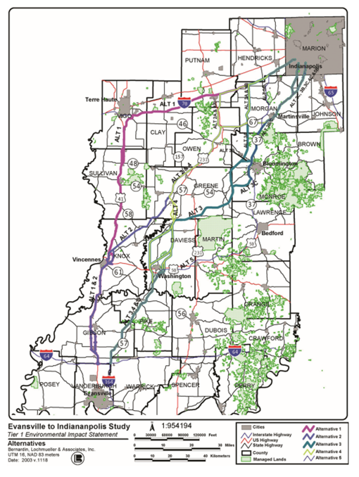
Source: INDOT (2018)
The qualitative discussion noted the potential sources and directionality of GHG effects and concluded with a comparison of total statewide emissions to global emissions:
As tailpipe and fuel cycle emissions generally increase with VMT, the project area would likely have an increase in GHG emissions under any of the build alternatives compared to the no-build scenario. Some of the increase in GHG emissions could be offset due to increases in speeds and reductions in congestion (which are associated with lower GHG emissions). Construction of the project would also generate GHG emissions. Preparation of the roadway corridor (e.g., earth-moving activities) involves a considerable amount of energy consumption and resulting GHG emissions. Manufacture of the construction materials and fuel used by construction equipment also contribute GHG emissions… Based on projections from the Energy Information Administration, CO2 emissions from motor vehicles in the entire state of Indiana contributed less than two tenths of one percent of global emissions in 2010.[5]
INDOT (2018)
4.9.5 Washington State DOT and the I-5 Columbia River Crossing: Quantitative Assessment
Since 2009, the Washington State DOT (WSDOT) has provided guidance for project-level greenhouse gas evaluations under NEPA and the State Environmental Policy Act (Washington State DOT 2018). Typically, EIS and EA projects require a quantitative analysis, while CEs require no analysis or a brief qualitative discussion. Quantitative analysis may include a quantitative planning-level GHG analysis, which is referenced in the project environmental document. When a project-specific quantitative analysis is performed, it must include operational (including tailpipe and upstream or fuel-cycle) emissions as well as construction and maintenance emissions.
If no planning-level analysis is available, the analysis must be conducted at the project level. A project-level analysis should use the most current version of the MOVES model for operational emissions. Fuel-cycle emissions are calculated using a fuel-cycle factor of 0.27 per FHWA guidance. Project-level construction and maintenance emissions should be calculated using FHWA’s ICE tool.
The analysis is typically documented in the Air Quality Discipline Report (for an EA) or the Energy Discipline Report (for an EIS), which are provided as an appendix to the environmental document. A summary is provided in the Cumulative Effects section of the main body of the EA or EIS. Template language is provided. WSDOT and Oregon DOT jointly developed an EIS for the I-5 Columbia River Crossing project (Washington State DOT and Oregon DOT 2011), which considered multimodal improvement options (Figure 4‑10). This was a large project with unusually detailed data available.
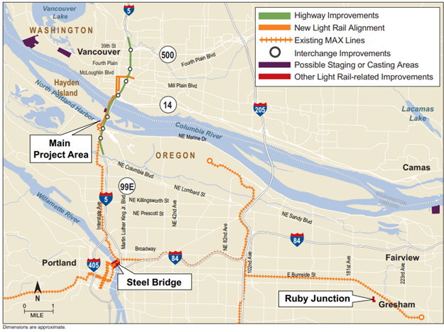
Source: Washington State DOT and Oregon DOT (2011)
Emissions from on-road vehicles and light rail were quantified at both the macro-scale (regional) and micro-scale (12-mile segment of I-5) using a variety of tools, including the regional travel demand model, a microsimulation model, MOVES, and eGRID. The locally preferred alternative was estimated to reduce emissions in 2030 compared to the no-build, with a quantitative comparison shown in Table 4‑12. The EIS concluded that based on the best available science and best practice GHG emissions measurement and modeling, the locally preferred alternative would result in a net reduction of GHG emissions compared to the no-build alternative. Note that comparing the change at a regional scale, rather than just for the project corridor, results in an absolute emissions reduction over six times as large, but a much smaller proportional reduction relative to total regional emissions.
Table 4-12. I-5 Columbia River Crossing GHG Emissions
| Scale | 2030 CO2e Emissions: No-Build (MT) | 2030 CO2e Emissions: LPA (MT) | Difference, LPA vs. No-Build (MT) | Percent Difference |
| Macro | 24,876 | 24,746 | -130 | -0.5% |
| Micro | 389 | 368 | -21 | -5.4% |
Source: Washington State DOT and Oregon DOT (2011)
4.9.6 Maryland DOT and the I-495 & I-270 Managed Lanes Study: Quantitative Assessment
Maryland DOT has not developed guidance for project-specific GHG emissions evaluation; however, the agency has had a Climate Action Plan in place since 2009 and annually reports on emission reduction activities.
The draft EIS for the I-495 & I-270 Managed Lanes Study (Maryland DOT 2020b) considered alternatives that address roadway congestion within the study scope of 48 miles from I-495 to south of the George Washington Memorial Parkway in Fairfax County, Virginia, to west of MD 5, and along I-270 from I-495 to north of I-370. The study alternatives included various combinations of high-occupancy/toll and high-occupancy vehicle lanes.
The scope of the GHG analysis included roadway links “that could significantly impact the study area.” The study area was defined differently for each alternative. Over a dozen alternatives were evaluated, with emissions quantified for six alternatives. The affected network and VMT changes were determined using the Metropolitan Washington Council of Governments regional travel demand model; emissions were modeled using MOVES at the county level. Emissions were modeled for 2015, 2025, and 2040, with linear interpolation of emissions in intermediate years shown in a figure. Figure 4‑11 provides an excerpt of a summary table from the draft EIS showing the projected annual CO2 equivalent emissions (percent change) and related factors on the “affected network.” Note that the no-build condition is different for each alternative since the study area was defined differently for each alternative. Construction emissions (reported in the final EIS, but not the draft) were modeled using the FHWA ICE tool. These emissions were reported as both total and annualized emissions over the 30-year project lifespan. Emissions were broken out for materials, transportation, construction, and operations and maintenance, and compared with usage (vehicle operations). The total of construction-related emissions was about 1 percent of vehicle operating emissions (Maryland DOT 2022).
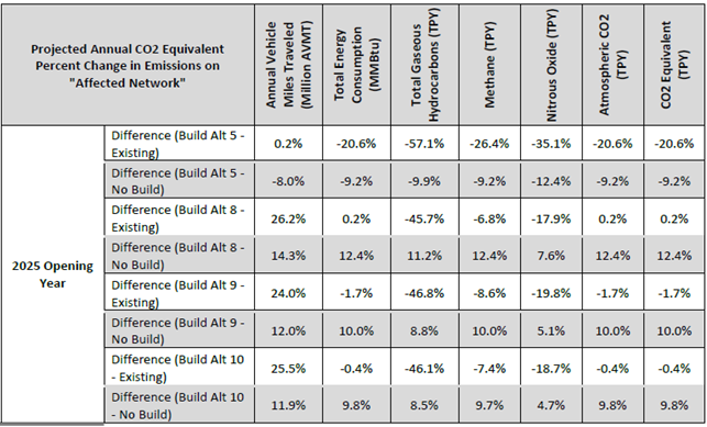
Source: Maryland DOT (2020b). Note that the final EIS (Maryland DOT 2022) modeled horizon year results for 2045 and only for the Preferred Alternative vs. No-Build.
The final EIS concluded that
…The proposed action is relatively minor in scope compared to the larger set of highway VMT and onroad mobile source GHG emissions that were assessed in a 2020 statewide (GHG) analysis. Highway capacity expansion projects can reduce emissions by reducing congestion but may also lead to increased VMT which can increase emissions and can also create additional emissions related to construction and maintenance. However, the emissions for this individual project would be expected to be much less than the collective total of all planned statewide projects and existing on road GHG emissions.
Maryland DOT (2022)
[1] Public Law 91–190 as amended through P.L. 118–5, Section 102 (C).
[2] MOVES4, released in 2023, reflects additional standards including the U.S. EPA light-duty GHG rule covering model years 2023 – 2026, as well as removal of the 2016 heavy-duty GHG rule’s trailer standards, which were vacated by a 2021 appeals court ruling. MOVES4 also includes improved estimates of energy consumption for EVs (EPA 2023). As of this writing, an updated technical document for GHG and energy consumption rates for MOVES4 has not been published.
[3] Council on Environmental Quality (2011). “Memorandum for Heads of Federal Departments and Agencies.” https://ceq.doe.gov/docs/ceq-regulations-and-guidance/Mitigation_and_Monitoring_Guidance_14Jan2011.pdf
[4] FHWA (undated). NEPA Transportation Decisionmaking. https://www.environment.fhwa.dot.gov/nepa/trans_decisionmaking.aspx
[5] As noted in Section 2.5, note that U.S. EPA and CEQ both caution against making such comparisons with global emissions.